graphs

Recidivism rates of US prisoners - reduced color palette
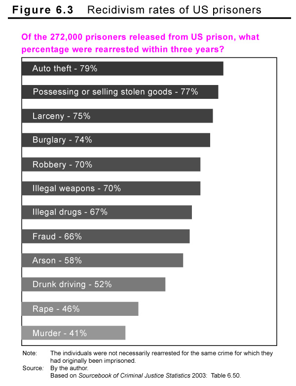
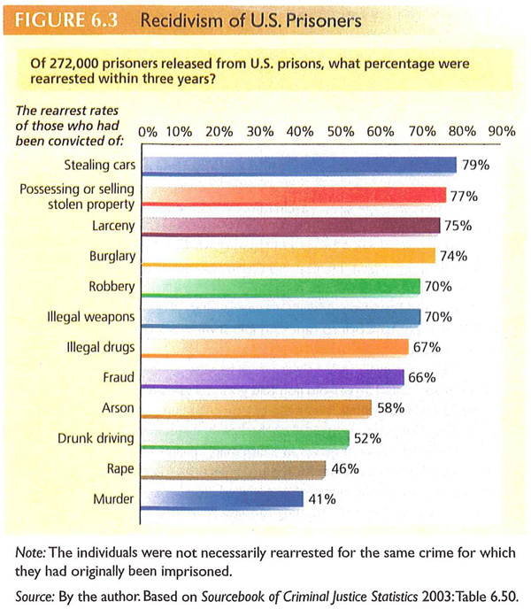
Figure 6.3 from Henslin's Intro to Soc - Recidivism of US Prisoners

On color

When architects draft plans and sections, they pay close attention to line weight. Part of the craft of draftsmanship is knowing which line weights are just right and making sure to apply the right line weight in the right instance. One of the criticisms older architects who were used to drafting boards and pencils levied against younger architects who draft using AutoCAD programs is that they just don’t do line weights properly. CAD displays layers in different colors and the younger architects were happy to rely on the appearance of these different colors as they worked on their monitors without making smart choices about line weights. When the documents were printed, all the lines could be the same weight, or if there were different line weights, they appeared to be arbitrarily chosen. Why were the older architects so upset? Because line weight carries meaning in architectural drawings. Get it right, and a simple section can speak volumes to the trained eye. Get it wrong and it’s like hearing a sentence without inflection (or perhaps worse, with inflections in the wrong places).

I feel the same way about color that the older architects feel about line weight. Color should mean something in a graphic. When the paint bucket comes out, there better be a reason for it beyond ‘decoration’. Graphic design is not about decorating otherwise drab diagrams. It is about enhancing the amount of information that can be communicated that privileges the image over the word because words always already require translation and the potential for misunderstanding.

The two bar graphs above depict the same information. One uses color with no apparent meaning attached to it – the bars are different colors just because it looks nice. The backdrop is yellow perhaps “to make the graphic jump off the page”. In my opinion, the full bleed back drop is like a heavy cloak, burying the information the chart contains in a Halloween costume. This Halloween celebration continues with the use of randomly selected colors for each bar on the chart. And the use of italics and bold where it isn’t needed is much like costume jewelry.

The gray-scale graphic uses color to highlight the originating question for the graphic. Each of the bars is shaded in accordance with the recidivism level for that crime – those imprisoned for auto theft have a 79% chance of being rearrested so that bar is 79% saturated with black. The bottom bar represents a 41% rearrest rate so it is 41% saturated with black. In this way, the saturation level reinforces the length of the bar and the numerical value printed in the bar.

References

Color graphic from: Henslin, James. (2009) Essentials of Sociology: A down-to-earth approach 8th ed., Pearson Publishing: New Jersey. Figure 6.3.

Gray-scale graphic: By Norén.

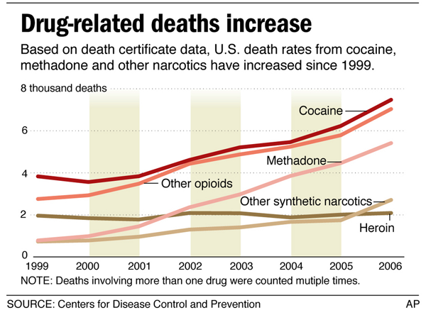
Drug related deaths increase - Associated Press article based on CDC data

What works

A simple line graph shows that more people are dying from methadone than heroin and the difference is growing over time. It also shows that cocaine is more dangerous than anything other drugs on the graph, at least when it comes to fatalities. Note that these data represent deaths due to acute overdoses as well as fatalities due to complications from long term use.

What needs work

I have no idea what the bars behind the line graphs represent. They seem to be there just to be graphic – I am not in favor of the use of meaningless graphic dross. The article that accompanied this graph mentions that 39,000 people die every year due to drugs and 45,000 die in traffic accidents (though auto-deaths are dropping and were at ~37,000 in 2008 according to Fatality Analysis Reporting System). This means that in some states – mostly in New England and the Mid-Atlantic – more people are dying from drugs than cars. This is big in America where traffic fatalities have long been an unfortunate fact of life. Safety standards have been improving so traffic deaths have fallen. I would have liked to see the traffic deaths applied to this graphic. It would have been more meaningful in the context of the article than the random bars behind the lines.

Where are alcohol related deaths?

The labels go from the very specific “Methodone” to the incredibly vague “other synthetic narcotics” and “other opioids”. The article says that the growth in drug-related fatalities is coming from prescription drugs like Oxycontin, Vicodin, and Methadone. OxyContin and Vicodin contain hydrocodone which places them in the “other opioids” category but it seems like it would also place them in the “other synthetic narcotics” category.

There are plenty of people who will not read the whole article. The graphic needs to speak for itself with clarity, complexity, and completeness otherwise it risks oversimplification and obfuscation.

Bonus graph

Oxycodone in grams distributed per 100,000 Population, Arizona and US, 1997-2006

The Proceedings of the Community Epidemiology Work Group, January 2009 included a presentation by James Cunningham that featured this data about the increase of oxycodone across the US population. I think this graph helps contextualize the oddly stylized line graph that is the central focus of this post. Here you can see that there is simply much more hydrocodone around than there used to be. The original article by the AP attributes this to the recognition of the treatment of chronic pain as a new and challenging medical field. In that case, then, it should be no surprise that Arizona is a hotbed for hydrocodone prescriptions because the state’s demographic is over-represented by the elderly who are more likely to need pain management strategies.

Final question

I don’t usually get political, and I’ll probably regret posing this question, but here goes.

Do drug companies bear any responsibility for the fatalities involving prescription drugs? Clearly it is in their financial interest to sell an addictive product – and nobody denies that opioids are addictive. Big tobacco ended up having to pay out millions, but that’s because in the beginning, they denied that their products were so unhealthy that using them was potentially fatal. Opioid producers are not making claims one way or the other on the question of fatality beyond admission that the substances are addictive and should be monitored by doctors. This shifts the blame to doctors, but it is often the case that addicted patients will seek these drugs from all sorts of different doctors making it difficult for any given doctor to know just what the patient was prescribed by some other health care professional. It is important to note that opioids offer meaningful treatment for chronic pain where tobacco products did not play a legitimate roll in mainstream medicine and thus should not be banned or taxed, etc.

This brings us back to the original question: should big pharma take some responsibility for deaths due to use/abuse of the prescription drugs from which they derive profit?

References

Associated Press. (2009, September 30) In 16 states, drug deaths overtake traffic fatalities at cleveland.com

A bigger version of the graphic is here: Drug-related deaths increase

Hydrocodone fast facts from drug-addiction.com

Community Epidemiology Working Group. (2009, January) Epidemiologic Trends in Drug Abuse: Proceedings of the Community Epidemiology Working Group | Highlights and Executive Summary [PDF] US Department of Health and Human Services, National Institutes of Health.

United States Literacy Rates - National Assessment of Adult Literacy

The key

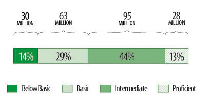
Number of Adults in Each Prose Literacy Level

Prose Literacy

* Below Basic:
o no more than the most simple and concrete literacy skills
* Basic:
o can perform simple and everyday literacy activities
* Intermediate:
o can perform moderately challenging literacy activities
* Proficient:
o can perform complex and challenging literacy activities

What works

This is a simple way to do a bar graph when all of your bars will add up to 100%. Just think: they could have laid this information out in a standard bar graph with a separate bar for each level of literacy. This way, it’s easier to see that all these parts add up to a whole population.

It is alarming that there are more people ‘below basic’ than ‘proficient’ especially in the increasingly text-based world we live in. Emails and chat clients have replaced many phone calls which is especially critical for workers. (I wonder if on a per-communication basis it costs more to use the phone. Anyone seen data?)

What needs work

I would have tried to get the categories labeled within the graphic itself. Referring to a bulleted list is a bit cumbersome. On the other hand, I appreciate the desire to thoroughly describe what each categorical label actually means, and it would have been hard to elegantly place all those words into the graphic.

References

National Assessment of Adult Literacy. (2003) Demographics overall.

Infant mortality gap between blacks and whites in Wisconsin

What works

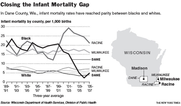
I like the inset map. Architects often include a small site map in the main exterior section of a new building to help the viewer understand where the building is in relation to the rest of the world. News programs often start out international stories with maps. I love that this line graph comes with an orienting map. I might have included just a shadow of some neighboring states simply because many Americans have only a fuzzy idea of where Wisconsin is. Sad but true.

The lines show a great deal of information, some of which is not addressed in the article. Quoting the main thrust of the article:
“Here in Dane County, Wis., which includes Madison, the implausible has happened: the rate of infant deaths among blacks plummeted between the 1990s and the current decade, from an average of 19 deaths per thousand births to, in recent years, fewer than 5. The steep decline, reaching parity with whites, is particularly intriguing, experts say, because obstetrical services for low-income women in the county have not changed that much.”

Then it goes on to quote a local doctor and professor: ““This kind of dramatic elimination of the black-white gap in a short period has never been seen,” Dr. Philip M. Farrell, professor of pediatrics and former dean of the University of Wisconsin School of Medicine and Public Health, said of the progress in Dane County. “We don’t have a medical model to explain it,” Dr. Farrell added, explaining that no significant changes had occurred in the extent of prenatal care or in medical technology.”

The graph suggests an explanation that the article (and the doctor) may not have considered. Presenting information visually is about more than presentation; rearranging data to reveal patterns is a research tool in itself.

What needs work

This is a critique of the article, based on the line graph: isn’t it possible that the at-risk folks in Dane County ended up moving to Racine for some reason? Right at the time the infant mortality rate in Dane was plummeting, the rate in Racine was spiking. From the line graph it seems that this happened in the vicinity of Clinton era welfare reform. Maybe there were some reasons for the most at-risk folks to get out of Dane and into Racine at this time.

If there is no medical explanation, let’s have a look at other possible explanations.

References

Eckholm, Eric. (2009, November 26) Trying to Explain a Drop in Infant Mortality The New York Times US Section, reporting from Madison, WI.

feltron graphic:  cnn.com site traffic since launch day
cnn.com site traffic since launch day

What Works

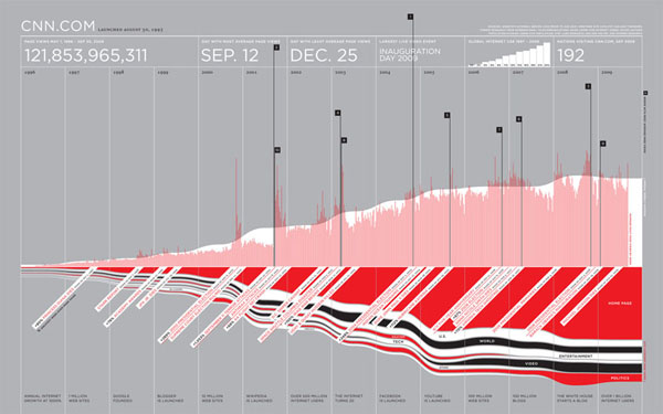
Think about what this graphic could have been: basically just a line graph showing growth over time. Now look at it again. The little flags point out cnn.com’s busiest days and remind you what was happening on those days – Obama’s inauguration, the September 11th attacks, various other political happenings. Even if this graphic weren’t labeled ‘cnn.com’ I bet you would have been able to predict it was a news site just by looking at which days it had the most hits.

Other things to like: the little graph at the top showing global internet use to remind us that the growth of page views per day could largely be a function of the growing number of people who have access to the internet rather than an inherent growth in popularity of cnn.com. Of course, the little bitty bar graph isn’t big enough to see if there is a difference in the growth rate in access to the internet overall and the growth rate in page hits at cnn.com.

Mirroring the trend over the x axis is a brilliant move here. On top, we see the page views per day averaged over the week in red and the annual weekly average. This allows them to go granular with their highest hit days and also give a trend line that smooths over the outliers. Nice. And on the bottom, then, they can show basically the same trendline broken into content areas. So if you’re a skeptic and you think all this growth is probably in entertainment because folks are just nitwits feasting on celebrity-ism, well, you can see that the home page gets by far more traffic than the entertainment page. It’s possible that the nitwit theory holds, but folks aren’t turning to cnn for juicy gossip. We can also see that video takes off and politics has more page views in election years.

And on Christmas, the number of people ignoring cnn peaks.

From Feltron, the graphic’s designer, the best thing about the narrative depicted by this graphic is the trust we all put in the internet as a reliable source of news after 11 September. “Ultimately, I think the most fascinating story here is the change in our news habits after September 11, 2001. After this day, a new and higher baseline for visits to the site is established, and the inference is that this event really established CNN.com and the greater Internet as a reliable, timely and indispensable source for news.”

What needs work

This is a sophisticated, well developed graphic that basically needs no work.

But…

The text is too small to read. Of course, it’s virtually impossible to create a graphic with this much detail that is elegant and uncluttered with text that fits in 800 x 800 pixels, or thereabouts. For folks who happened to have the ever widening monitors, it would have been nice to link to a ginormous version. I bet feltron has a larger version since I’m not sure how he would have been able to convince himself that some of the smallest text was legible otherwise.

References

Feltron (2009, 11 November) cnn.com traffic graphic on Feltron’s blog at tumblr.com.

Charles Blow's graphs to track voter apathy by age group

What needs work

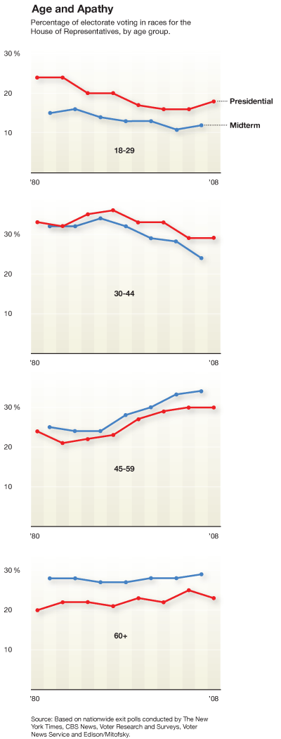
These graphs are meant to illustrate voter apathy by age group.

Jay Livingston, blogger at Montclair socioblog, points out that comparisons between age groups would be far easier if all the age groups appeared on one graph. I agree.

I would also point out that I’m curious about whether it is strictly age or a cohort effect that is really at the heart of the question about who votes. In order to answer that by using infographics, I might have looked at voting rates within cohorts over time (so graph the baby boomers voting rates as they age and so forth).

One picky little detail: when making graphs that have to do with voting, it’s probably best to assume many people will see red and blue and think Republican and Democrat. I would have preferred any other colors, just to avoid confusion.

The bigger problem

Folks, leave your computer alone for a minute and vote.

References

Blow, Charles. (2009, 14 November) “The Passion of the Right” op-ed in the New York Times.

Michael Schwabs poster design for the Art Center College of Design in Pasadena, CA

How to go from inspiration to design?

There are plenty of great graphic designers plastering walls with posters, filling magazines with intelligent ads, and even getting their work into museums. A lot of the time, it’s hard to see how all the inspiration and excitement of graphic design for advertising can make it’s way into the information graphics social scientists use to communicate their findings.

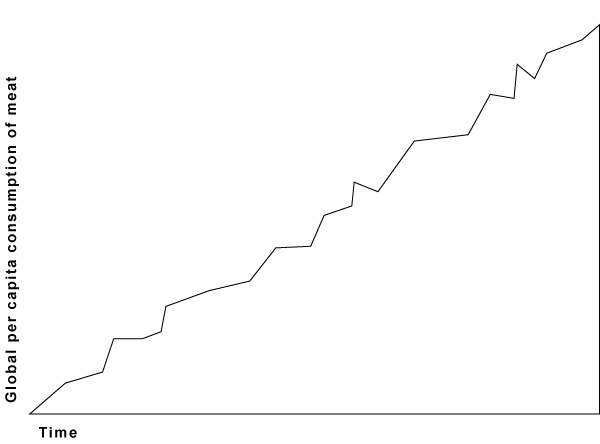
I took a fake example to show you how I translated my appreciation for Schwab’s design into some thoughts about enlivening a basic line graph. Let me emphasize this one more time: this example is fake. I didn’t use real data. Yes, global consumption of meat is increasing per capita, but no, it’s not as dramatic at it appears here. I went ahead and left off scales on the X and Y axes to ensure this graphic doesn’t end up traveling around the interwebs as truth.

Step 1

Break down Schwab’s graphic. He’s basically got a right triangle sitting on a single color background that bleeds into a thick border. The border contains the only text. The only realist element – the pencil – intersects the triangle to make what is like a giant X in the center of the poster.

How is this at all like social science graphics? Well, if you flip the triangle, it’s a lot like any positive relationship as depicted by a line graph.

Basic positive relationship depicted by a line graph

What next?

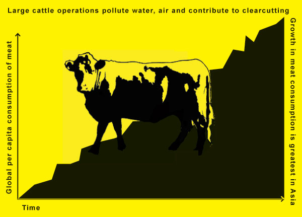
Now that you can see how a line graph is a little like Michael Schwab’s elegant pencil poster we can start to apply his decisions directly to our graphic. First, we can add a clearer background. If it’s just white the thick borders do not read as thick borders. They just look like the same old place everyone puts their axial labels. I distinguish this by adding a background color which will pull the borders into a relationship with the background behind the graph. I also go ahead and fill in the area under the graph to help nudge it into reading as an area, rather than some jiggly line.

The tough part here is the graphic. Not all stories we want to tell are going to be linked to a slender X-making image. I chose to depict the rise in meat consumption. Sure, I could have picked a cattle prod or other cattle killing tool dripping with blood. It would have been slender and I could have made an X. But I was trying not to appear unbiased so I just went with an iconic image of a beef cow. I planted the cow in the middle. We do lose a few data points in the middle – there are ways to deal with that if it’s important (overlay a yellow line across our cow’s gut where the data points are missing).

Here’s what we’ve got. The point is that the graphic below is the basically the same data as our line graph above except far more arresting (I took the liberty of adding two more lines of text – not necessary, but I was trying to closely follow Schwab’s concept). If you are trying to keep the attention of the audience in a presentation, be they sleepy students or sleepy colleagues, it might be worth your while to take a little extra time on your most important graphics. And if you do have one or two major points you want the people to take away from the graphic, you can write them across the top or up the side. Writing up the side is not as good – use it only for secondary points or graphic credits in the case that you hire someone to craft your graphics.

Simple line graph copying Michael Schwab's concept

References

Schwab, Michael. (2009) “Instrument of Creativity” [poster design] Art Center College of Design in Pasadena, CA.

Hirasuna, Delphine. (2009) “Art Center’s Instrument of Creativity” in At Issue Journal: The Online Journal of Business and Design. San Francisco, CA.

CEO Compensation 1970-2000 (Conley, D.)

What Works

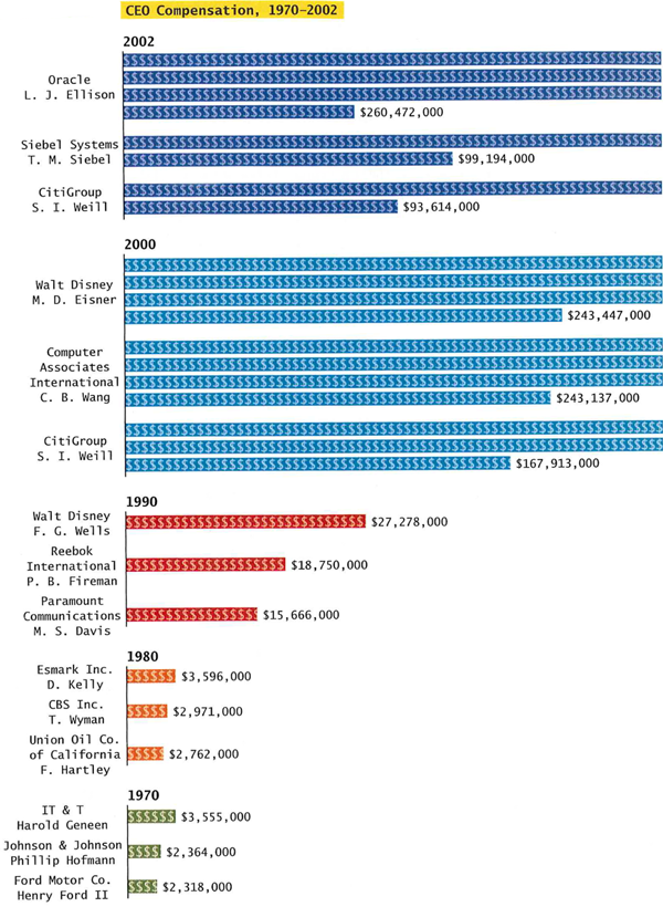
This is a great concept because CEO compensation has ballooned relative to compensation for the rest of us.

What Needs Work

I would like to see some of the comparative data on compensation for the rest of the work force somehow, not just CEOs.

It would be nice for the graphic to say that the figures are all in year 2000 dollars.

Collapsing the bars instead of stringing them out diminishes the visual impact dramatically. If the highest compensation was displayed end-to-end instead of broken up and stacked it would look far more disparate compared to the 1970 compensation data. Now, realizing that this would skew the page layout, the graphic designer could have pursued a volumetric portrayal instead of just a two dimensional version.

Relevant Resources

Conley, D. (2008) You may ask yourself: An introduction to thinking like a sociologist New York: W.W. Norton & Company. p. 563.

immigrants_suburbs_sm

What Works

This is beautiful. Just look at it and tell yourself why it works. Think about how crappy it would have been if all the cities had been crammed on to one graph. Stringing them out like this, one city per graph, tells the story of immigrants moving to the suburbs so elegantly. The density increases from left to right with time series adequately represented for each city.

Relevant Resources

DeParle, Jason. (2009 April 28) Struggling to Rise in Suburbs Where Failing Means Fitting In New York Times, part of the Remade in America series.

Water Resources and Withdrawals by Continent

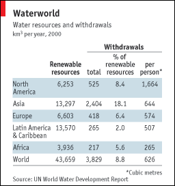
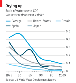
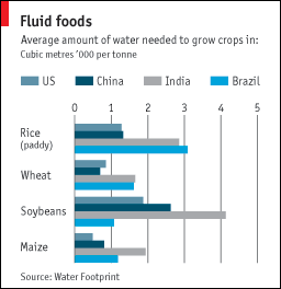
These graphics accompanied a great article about water shortages in episode of The Economist which arrived last week. The article was well written and comprehensive, handily summing up the way water resources are related to the growth of urban centers, climate change, the rising affluence of the world’s poorest people (and their conversion from vegetarianism to omnivorousness) and the question of whether or not fresh water is a global or a local problem. I highly recommend reading it. Unfortunately, I think you would do almost as well reading it without the accompanying graphics as with them.

The first one is so confusing I still don’t know what I am seeing here. Table data usually has the attribute that the longer you look at it, the more you get, with an occasionally painfully long initialization period in which you can’t make out any pattern whatsoever. I spent a good bit of time on this one and I still don’t know how to make sense of it. The article rightly points out that fresh water is unevenly distributed across the globe–some places have a lot, some places hardly have any. No big surprise. Also not surprising: some continents use more fresh water than others based on overall population size and agricultural production practices. So when I looked at this graphic, I was kind of hoping to get a sense of both how efficient each continent was with their resources and how dire their straits were. The graphic sort of does that. Sort of. We’ve got a measure of total renewable water resources but it doesn’t take into account total land area. It does take into account population, sort of, and maybe population is more relevant than total land area in this case.

Ratio of Water Use to GDP

The second graphic does not stand well on it’s own. I can see here that it appears that these selected countries seem to have been becoming more efficient with their water use. Since 1995, all of these countries have lowered the number of cubic metres of water used per dollar (or dollar equivalent) of GDP. This graphic does nothing on its own to help me understand why that might be true. Have these countries moved out of water intensive agricultural production? Have they made their agricultural production more efficient? If so, is it technological change leading to increased efficiency or did they just shift to more efficient crops? Or maybe the change is in the GDP variable, not the water variable. The graphic really just doesn’t clear any of these things up.

What Works

Water Used to Grow the Same Crop in Different Countries

I like the third graphic. It’s clear and adds to the text in the article. This isn’t the first time I have read about water shortages and one of the biggest and possibly easiest changes we could make to prevent the water shortage from becoming any more of a problem than it already is, would be to introduce drip irrigation in places that do not already have it. Yes, it costs some money. But it is far more cost effective than many of the other strategies introduced to combat climate change. Drip irrigation technology is not overly complex nor does it require extensive training or equipment to install. Tubing perforated along its length with small holes, buried under the surface of the earth, delivers water directly to plant roots. Much less water is lost to evaporation or seepage into non-crop areas. Control over water resources is better – during rains cisterns collect and store water for later distribution through the drip tubing during dry periods.

Relevant Resources

The Economist. (2009, 8 April) Water shortages go global: Sin aqua non. Istanbul.