housing

Housing vacancy rate in Wisconsin, 2010
Housing vacancy rate in Wisconsin, 2010 | Jan Willem Tulp

What works

The “Ghost Counties” interactive visualization by Jan Willem Tulp that I review in this post won the Eyeo Festival at the Walker Art Center last year. The challenge set forth by the Eyeo Festival committee in 2011 (for the Festival happening in 2012) was to use Census 2010 data to create a visualization using Census data that did not rely on maps…or if it did rely on maps, it had to use maps in a highly innovative way. This is an excellent design program – maps are over-used. Yet it’s one thing to assert that maps are over-used and another thing to produce an innovative graphic representation that is not a map.

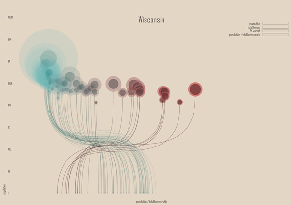
Tulp does a great job of leaving the map behind. He also does a phenomenal job of incorporating a large dataset (8 Mb of data serve the images in the interactive graphic from which the stills in this post were captured). The graphic has a snappy response time once it has loaded and his work makes a solid case for the beautiful union of large data and clear representation thereof.

The color scheme is great and reveals itself without a key. Those counties with low vacancy are teal, those sort of in the middle are grey-green, and those with high vacancy are maroon. The background is light, but not white. White would have been too stark – like an anesthetized space. He experimented with darker backgrounds (see his other options at his flickr stream here) but those ended up presenting an outer space feel. The background color he settled on was (and is) the best choice. Background colors set the tone for the entire graphic, along with the font color, and Tulp’s work is positive evidence of the value of carefully considering them.

Pie charts might be better than circles-in-circles

The dot within a dot is difficult for the eye to measure. Pie charts- which I only recommend if there are very few wedges – would have worked well with this type of data because there are only two wedges (see here for an example of a two wedged pie chart). I just finished reading Alberto Cairo’s important new book The functional art and he had a solid critique of the circle-in-circle approach that helped me realize what’s so appealing, but just plain wrong, about circles-in-circles:

“Bubbles are misleading. They make you underestimate difference….If the bubbles have no functional purpose, why not design a simple and honest table? Because circles look good. (emphasis in original)”

In this case, a wedge in a pie chart could have represented the percent of total housing units occupied.

Why is it so hard to ‘see’ rural vs. urban?

The x-axis is a log scale for population size. It’s clear from what we know about the general trend towards urbanization that we would expect urban areas to have lower vacancy rates than rural areas. Even in 1990 – two census surveys before the 2010 data that was used here – the New York Times ran a story about the population decline in rural America and there has been widespread coverage of the trend towards urbanization by both journalists and academics (the LSE Cities program does nice work).

Housing vacancy rate in Minnesota, 2010
Housing vacancy rate in Minnesota, 2010 | Jan Willem Tulp
Housing vacancy rate in New York, 2010
Housing vacancy rate in New York, 2010 | Jan Willem Tulp

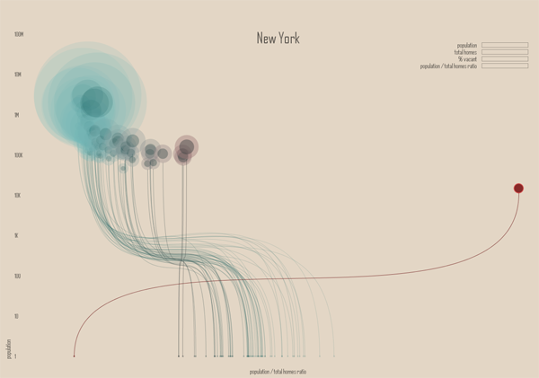
The two states shown here – New York and Minnesota – both have some big cities and a whole of small cities in rural areas. Some small cities are also in suburban areas. That’s a problem with this visualization, the distinctions that have been established in academic literature between rural, suburban, ex-urban, and urban are difficult to pick out of this visual scheme. While it would be difficult to find a sociologist who could wrangle the data to produce this kind of visualization, I imagine many of my intellectual kin would be confused by this visual scheme and demand to return to a map-based graphic because at least in that case they could see patterns associated with the rural-urban spectrum the old-fashioned way. I am not wedded to the notion that a map is the only way to “see” the rural-urban spectrum, but the current configuration makes it difficult to think with the existing literature about housing patterns even though the attempt to distinguish between population size was built into the graphic on the x-axis. Population size is not always a great proxy for urban vs. rural, so it is a weak operationalization of spatial concepts social scientists have found to be meaningful. For instance, a small, exclusive ex-urban area filled with wealthy folks and their swimming pools is conceptually much different from a small, depopulating rural town even if they have roughly similar population sizes.

It is important in a research community to build on good existing work and reveal the weaknesses of existing work where it’s falling short. Either way, it is a bad idea to ignore existing work. Where a project does not relate to existing work – neither building momentum in a positive direction nor steering intellectual growth away from blind alleys – it will likely become an orphan. In this case, the project is only an orphan with respect to urban scholarship. As a computational challenge, it most definitely advanced the field of web-based interactive visualization of large datasets. As a visual representation, it adhered to a design aesthetic that I would like to see more of in academic work. But as a sociological analysis, it’s nearly impossible to ‘see’ clearly or with new eyes any of the existing questions around housing patterns. It is also my opinion – and this is far more easily contested – that it does not raise new important questions about housing patterns in urban, suburban, or rural America either.

My critique here is not that all data visualization is pretty but useless and that we should stick to our maps because they tie us to our existing disciplines and silos of knowledge. Rather, my critique is that in order for data visualization to become a useful tool in the analytical and communication toolkits of social scientists, the work of social science is going to have to find a way into the data visualization community. As anyone who has tried to use Census data knows, looking at piles of data is not synonymous with analysis. While Tulp’s graphics certainly present an analysis, that analysis seems to have turned its back on a fairly sizable swath of journalism on urbanization, not to mention the hefty body of academic work on the same set of topics.

Graphic Sociology exists in part to find a way to keep social scientists motivated to produce higher quality infographics and data visualizations than what is currently standard in our field. But the blog is equally good for sharing a social scientific perspective with computer scientists and designers who are ahead of us with respect to the visual analysis and display of social data. There is a way to bring the strengths of these fields together in a meaningful, positive way. We are not there yet.

References

Cairo, Albert. (2013) “The Functional Art: An introduction to information graphics and visualization.” Berkeley: New Riders.

Eyeo Festival.

Tulp, Jan Willem. (2011) “Ghost Counties” [Interactive Visualization] Submitted to Eyeo Festival and selected the winner in 2012.
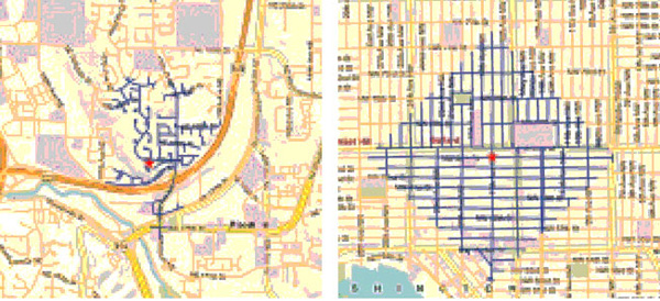
Second Trimester 2010 Rental Prices in Madrid
Second Trimester 2010 Rental Prices in Madrid | idealista.com

What works

This idea is so simple and demonstrates the reason tables are great as well as the reason trend lines are great. In general, tables are capable of organizing more information than most information graphics. Sure, you can have small 2×2 tables but there can also be tables that go on almost to infinity (or so it seems if you are asked to turn them into an information graphic). But tables are extremely flexible and this is just one simple example of how they can accommodate trend lines.

The folks at idealista.com prepared a report covering second trimester rental prices in Spain and above you can see what has been going on in the neighborhoods of Madrid. They include the numbers as well as trend lines that demonstrate in a glance the recent history of prices in those neighborhoods. It isn’t rocket science to stick those trend lines right in the table, but it is useful. This should also remind all of us that trend lines are legible even when they are very small.

What needs work

Those trend lines need at least a start date and an end date. It is tempting to think that they start at the beginning of the trimester and end of at the end of that trimester but it is unclear (and unlikely, in my opinion). Plus, some of the trend lines seem to start up in the middle rather than at the beginning.

Rental prices in Spain – 2010

In case you came to this blog because you are, in fact, concerned about housing rental prices in Spain, here’s a summary of the report. While there have been statistically significant but small price changes in some markets, in Madrid and Barcelona, rents are basically holding steady.

References

idealista.com (2010 16 July) Evolución del precio de la vivienda en alquiler [Rental housing price report]

Map comparison highlighting walking distances in urban grid vs. cul-de-sac layout
Cul-de-sac urban planning limits walking distances | Urban Design 4 Health

What works

This side by side comparison is meant to show the length of all possible paths from a given point, assuming a person walks for five minutes. (Or maybe it’s ten minutes, but you get the idea.) Because the grid goes on forever – remember calculus? a line is defined by two points in space but continues for infinite length – the length of linear X-minute walking paths is longer than the more ‘organic’ length of cul-de-sacs. Of course, in cities, we are not talking about the ideal typical infinite lines found in calculus nor are cul-de-sacs some naturally determined path based on where deer walked down to the stream to get water before developers plopped a suburb down in the same spot. Both the grid and the cul-de-sac based suburb are planned developments. The question has become (see references below for a small sample of the people who are asking it): is the grid better than cul-de-sacs?

The folks who constructed the graphic above are interested in fit cities. They want you to see that because cul-de-sacs make it much harder to walk (or bike) around the neighborhood, they might be contributing to car culture and, in the end, making us fat. Fit cities are the antidote to fat cities and there is much urban design being driven by our collective (and towering) BMI. Lawrence Frank, Bombardier Chair in Sustainable Transportation at the University of British Columbia gets his hands dirty researching this question and he found that, “neighborhoods in King County, Washington: Residents in areas with the most interconnected streets travel 26% fewer vehicle miles than those in areas with many cul-de-sacs.” Furthermore, “Recent studies by Frank and others show that as a neighborhood’s overall walkability increases, so does the amount of walking and biking—while per capita, air pollution and body mass index decrease.

Cul-de-sac illustration
Illustration by Lauren Nassef

I think the concept behind the above graphic is solid. It doesn’t do the best job at showing distances walked, but it does a great job of visually demonstrating general walkability. The grid is good at making space permeable; cul-de-sacs are good at making space rather impermeable. I would point out that everything could have been much cleaner if some of the information and colors in the background had been dropped out. A grey-scale representation of the available routes overlaid with the walking routes in color would have put some polish on the visual without altering the concept. Plus, I would have liked a key somewhere telling me if this is 5 or 10 minute walking distance.

What needs work

Collective fitness has only recently hit the urban planning scene as a concern foremost in designers’ minds. Back in the 1980s when crime rates tended to be higher, for example, there was a great deal of concern about safety. Shane Johnson and Kate Bowers did a similar comparison also setting cul-de-sacs up against the grid (sadly, without generating any infographics) but this time they were wondering if cul-de-sacs experienced fewer burglaries than linear streets. Before you get your panties in a snit about demographic issues like income that could impact both burglary rates and the likelihood of living in a cul-de-sac neighborhood, I’m telling you that Johnson and Bowers controlled for income. They also controlled for ethnic heterogeneity. They were not able to measure whether or not cul-de-sac neighbors were more likely to have home security systems. What did they find? Cul-de-sacs are safer – fewer burglaries. They point out that there could still be elements of cul-de-sac neighborhoods that have nothing to do with urban design that they weren’t able to fit in their statistical model. Feel free to read the paper and make your own decision, but I was compelled by the fact that even the presence of foot paths connecting cul-de-sac hoods tended to increase the incidence of burglaries.

Johnson and Bowers sum it up thus:

For this study area at least, the policy implications would seem to be quite clear; permeability should be limited to that necessary to facilitate local journeys and sustainable transportation. Additional connectivity may lead to elevated burglary risk and so should be avoided. Cul-de-sacs, in particular, would appear to be a beneficial design feature of urban areas and so should be encouraged.

Overall, then, I think the jury is still out on the question of cul-de-sacs. Perhaps the most important point is to note that like many other things – fashion, food, sport – scholarship has trends. The trend in urban design now focuses on public health, especially fitness. It used to be crime. Before that one might remember that fears of nuclear annihilation influenced design. I’m not picking on urban designers for being faddish. Trends flow through all disciplines with which I am familiar.

References

Johnson, Shane and Bowers, Kate. (Online | December 2009, Print | March 2010) Permeability and Burglary Risk: Are Cul-de-Sacs Safer? . Journal of Quantitative Criminology Vol. 26 (1).

Popken, Ben. (23 June 2010) Cul-de-sacs are making us fat at Consumerist.

New York Times Magazine. (2009) “Ninth Annual Year in Ideas: The Cul-de-Sac Ban”. [above illustration by Lauren Nassef].

New York Chapter of the American Institute of Architects. (2010) Fit City 5: Promoting Physical Activity Through Design” Architecture Lab.

Wieckowski, Ania. (May 2010) Back to the City in Harvard Business Review.

Private/Public: Rethinking design for the homeless
Constituency Chart

What works

What Terri Chiao and Deborah Grossberg Katz from Columbia University’s GSAPP design school have done is come up with a way to represent percentages using a flow-chart. Not only is it creative in the sense that this sort of data rarely gets displayed this way, but it helps turn the data into a narrative. In order to figure it out, the viewer quite literally has to reconstruct a story that sounded something like this in my head: “The population they are concerned about has 40% of people already experiencing homelessness with another 60% at risk of homelessness. The folks who are already homeless are the only ones living on the street, but really, 75% of already homeless people live in shelters. As for the at-risk-of-homelessness people, 60% live with family or friends. Twenty-five percent of the at-risk population owns their homes … why, then, are they at risk of homelessness? Both the at-risk and already homeless groups have far more families than single folks. And what does it mean to be homeless in jail/prison? That you aren’t sure where you will go when you exit? Somehow I feel like that could describe a lot of the prison population. And what about half-way houses? Those still exist, right?”

The flow-chart concept is not typically used to describe the breakdown of percentages and what works here is that it forces the viewer to walk through the narrative. As a pedagogical maneuver, it’s quite successful. Because of the way the information is presented, it invites questions in a way that a pie chart or a bar graph may not. It’s also a little harder to interpret. Graphics that invite questions often are a bit more challenging to ingest, not quite so perfectly sealed as other more common strategies might appear.

What needs work

I spent a good deal of time looking at this chart trying to figure out what the blue means. I still don’t understand what the blue means.

I also would like to see on the graphic some explanation of how they determined who was at risk of being homeless. Because when I got to the section of the flow-chart that showed how many of the at-risk population owned their homes, I began to get confused. By ‘own home’ do they not mean actually owning the home, but renting it or paying a mortgage on it? And if they do mean that folks actually own their homes outright, how can they be at risk of homelessness? Is the home about to be seized by eminent domain to make way for Atlantic Yards? At risk of being condemned (I hope NYC doesn’t have so many properties at risk of condemnation)? I’m sure if the makers of the graphic ever find their way to this page they will be upset because ‘at-riskness’ is described in the paper. But in life online, stuffing a little more text into the graphic is often a good idea because cheap folks like me will take the graphic out of context and whatever isn’t included will be lost. In this case, though, all is not lost. First, you can visit the blog on which I found this lovely graphic and get the whole story. But if you aren’t ready for all that, note that the authors define those who are at risk of homelessness as anyone who has spent some time in a shelter in the past year, regardless of whether they happened to have been homeless at the time of the survey.

Bonus Graphic

They also included the graphic below. I still don’t know what the blue means. This graphic does make it easier to understand that being truly homeless appears to mean running out of friends and family who have homes to share. Because none of the truly homeless live with family and friends. It’s also clear from both graphics that most homeless people are not visibly homeless. The folks you might see sleeping on the train or the street 1) may not be homeless, they could be sleeping away from home for reasons unrelated to homelessness per se and 2) if they are homeless, they may be quite different from the rest of the homeless population. They’re more likely to be single adults than families and more likely to be men than women.

Public/Private:  Project Sites
Public/Private: Project Sites

References

Chiao, Terri and Grossberg Katz, Deborah. (11 November 2009) “Public/Private: Rethinking Design for the Homeless” at Urban Omnibus.

US household size shrinks, living alone increases

Living Alone

I am helping a professor develop some graphics for his forthcoming book about the increase in people living alone. Above is just a rough draft; I’m still thinking about adding a border. Comments are welcome. More graphics coming in drips and dribbles.

References

US Census: Living Alone

Where does my money go? in the UK - Open Knowledge Foundation, raphic by Iconomical

What works

This visually arresting graphic does a great job of presenting data about national spending in an apolitical but altogether fascinating way. It’s interactive, by the way, but I’m not commenting on the interactive part, just the static graphic. I find that getting the static graphic clear is an important first step towards making a functional interactive graphic. If ever I hear someone say ‘but it’s interactive’ as an excuse for having a weak static graphic, I cringe. See my post about the USDA mypyramid food guide for a case study on the importance of a strong relationship between the static and interactive iterations of graphics as tools.

Each dot represents a different department or governmental program with the size corresponding to the funding level. Smart.

If you link through to the originating site, you’ll be able to follow blog posts that take readers through the development of the graphic. They ask for input and do their best to incorporate it. I like that approach. Good use of technology, OKF.

What needs work

I can’t quite tell why the circles are arranged the way they are or why their hues are the shades they are. Graphics, especially the beautiful ones, are the best when their simple clarity gives way to an elegant complexity. In other words, when I pose the question: “why does the hue vary within given funding types?” I’d like the graphic to lead me to an answer. I’m sure there is a reason for each hue, I just haven’t been able to figure it out.

One tiny, American-centric request: Add ‘UK’ to the page or the graphic somewhere. Maybe change “Total spending” to “Total UK spending”. Or “Where does my money go?” could be “Where do UK taxes go?”. These here interwebs are global. Yes, of course, the £ symbol tends to give it away. Maybe I’m just being too picky.

References

Open Knowledge Foundation. (2009) “Where does my money go?” United Kingdom. Data available

New York City - Upper East Side [from envisioning development]
New York City - Upper East Side {from the Center for Urban Pedagogy, envisioning development project}
New York City - East Harlem [from envisioning development]
New York City - East Harlem {from the Center for Urban Pedagogy, envisioning development project}

What works

Please click through to see the full affordable housing map of the New York City metropolitan area. The images above were generated using their pdf generator, but the full flash version is simply better.

Maps are hot. They’re everywhere. I was at a final presentation last night and one of the students said, “I’m kind of a map geek”. I didn’t realize it was possible to be a map geek, but I’m starting to understand. It’s quite easy to present a map – maps have been in use for centuries and some of the oldies are still goodies. It’s not so easy to combine a map with social science data in a smart, legible way. Folks try all the time. These folks at the Center for Urban Pedagogy got it right. Their affordable housing map tool is a solid example of the capability and execution of interactive data.

Why?

The map itself has been stylized. All they want to show you is neighborhood boundaries and neighborhood names. Gone are street markings, terrain, unnecessary color, landmarks, subway stops, and so on. They’re going to add some layers and your eyes are going to be better off without excess detail at the level of the map. Plus, they’re helping you to understand that it isn’t possible to get more granular than neighborhood masses. You can’t use this map to look at property values by block or by proximity to a subway stop so there’s no reason to include the subway map or street markings.

This grey massing approach helps focus my attention (and hopefully yours) on the layer of information about income by neighborhood. This information IS in color. It is added as a layer on top of the map without obscuring the map. They’ve used a modified bar graph layout in which information is embedded in the x-axis itself. The y-axis is implied – that’s just fine here.

And it’s interactive. In a good way.

From a technical perspective, this site makes good use of Flash. It loads quickly and is responsive. Once a neighborhood is selected the bar graphs realign themselves with colored blocks flying in from cyberspace to construct the balance of income for that neighborhood. Note that this is enough movement to make the whole experience a little exciting, a little sparkly but it doesn’t take so long to load or run that you’ve lost interest before you’ve gotten through it.

Layers.

It is my pedagogical opinion that the best graphics encourage the viewer to formulate a question which is then answered. In this case, what we see first is a neighborhood map. The viewer has to pick a neighborhood before any of the juicy data is revealed. This is great. Now, say, we’ve picked the Upper East Side and we see a towering skyscraper-like bar graph way over in the “High Income” department. Our next step can either be to compare to nearby neighborhoods, by clicking on East Harlem to the north, or to add the information about housing prices. The title is “What is affordable housing?” so clearly this is what the designers hope you’ll do. But they aren’t so impatient about it that they try to incorporate it into the first splash page.

References

Center for Urban Pedagogy. (fall 2009) Envisioning Development project. New York.