Search results for people living alone

What works

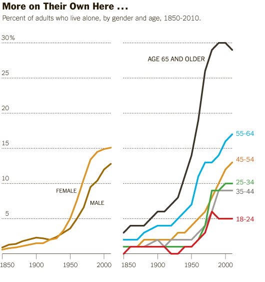
This post is an update to an earlier post about the increasing rate of Americans living alone. The first graph does an excellent job of visualizing the change in Americans’ tendencies to live alone, by age and gender. It’s clear that living alone is on the rise, especially for Americans over 45. It’s interesting that there seems to be a collective slow down in this trend in the decade between 35 and 45 when I suppose some of the late-to-marry people finally settle down and before the marital dissolution rate starts to fire up.

The graphics in this post accompanied an article by Eric Klinenberg in the New York Times Sunday Review that laid out the basic findings in his latest book, “Going Solo” that was based on 300 interviews with people living alone. He finds that while for some, living alone is an unwanted, unpleasant experience, most people who live alone are satisfied with their personal lives more often than not. In fact, they are more social, at least in some ways, than are their counter-parts who live with others. Singletons (his word, not mine. I prefer ‘solos’ in part because it’s an anagram), go to restaurants and other social spaces more often than do those who live with others.

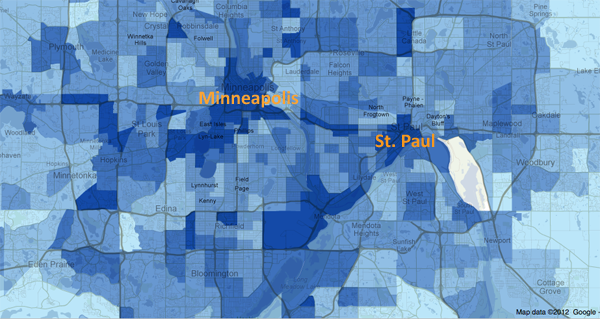
In a number of cities, including Minneapolis, more than 40% of households are single-people households. The article included an interactive map down to the census tract level that shows what percentage of households in that tract were single-person households in 2010. I took a look at Minneapolis and St. Paul and found that the map supported Klinenberg’s qualitative findings. The highest concentration of solos is in the center city areas where opportunities to get out and be social in the community are the highest. The suburbs and rural areas have fewer solos.

I encourage others to use the map and see if their local cities replicate this pattern, that more solos live in ‘happening’ areas than in quieter areas. Of course, this could be caused by a third variable, the presence of households that are affordable for single-earner households…but there isn’t enough analytical power in the map tool to be able to sort out the dependencies.

What needs work

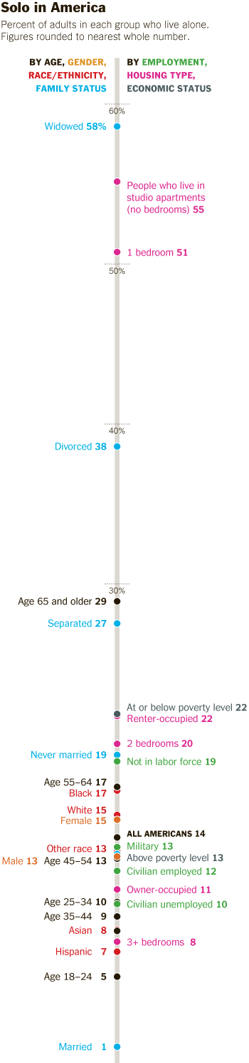
The information about who lives alone by age, marital status, and race that is displayed in the following long skinny stack of datapoints is the right kind of detailed information to use as an entrance into a deeper discussion about living alone, now that we’ve gotten a sense of the view from 30.000 feet. The problem is that this graphic is hard to read, too long for a single computer screen (but in order to make sense of it, one needs to see the whole thing at once), and too optimistic about what color differences are able to do than is reasonable.

The article does a better job of subtly navigating the movement from historical and international context into a detailed, robust analysis. By awkwardly pinning all the data points onto the stalk at once, viewers lose the ability to see patterns within data subsets. Here’s a test. Look at the following data and try to explain to yourself how race and living alone go together. Or how age and living alone go together. The graphic designer was hoping color would be able to do more than it has been able to accomplish here. The color is supposed to tunnel your vision down to a particular color-coded subset so that you can start to understand well just what it is about race or age or marital status that produces particular patterns in living alone. But I had a lot of trouble with the color frame because, quite literally, I had to keep shifting the frame around this graphic – it didn’t fit on my laptop screen. [Graphic designers often work on nice, roomy screens where they end up seeing more at once than their eventual audience who is probably peering at this thing from a web browser on a laptop or occupying half of a monitor somewhere.]

All the clustering around the mean is another problem that could have been avoided had the graphic been organized differently. As it is, all sorts of groups lump on top of one another down around 14%.

I also kind of hate that I can’t add categories together in any meaningful way here. I can tell that being a widow would put someone at high risk for living alone, but that’s kind of a no-brainer, isn’t it? I would have gotten more mileage out of visualizing the absolute numbers of people living alone by marital status, age, and race. Maybe over half of all widows live alone, but I haven’t the faintest idea how many widows there are in America so I don’t know if half of all widows is half a million people? Or 3 million people? Or whether it’s more or less than the 38% of separated people who are living alone. 19% of never married’s live alone, but because these people are likely to be young, maybe that is actually a larger absolute group than the 58% of widows living alone.

Final verdict: There was both a data fail and a graphic design fail.

References

Klinenberg, Eric. (2012) Going Solo: The Extraordinary Rise and Surprising Appeal of Living Alone. The Penguin Press HC.

Klinenberg, Eric. (2012) One’s a Crowd. New York Times Sunday Review.

Weber, Susan and Beveridge, Andrew. (2012) [infographics]
Solo in America graphic Line graph looking of the changing percentage of singleton households in America, 1850-2000
More on their own here…and even more abroad American and International singleton households.
Mapping the US Census: Percentage of Households with only one occupant Interactive graphic of US singleton households by census tract.

Living Alone

I am helping a professor develop some graphics for his forthcoming book about the increase in people living alone. Above is just a rough draft; I’m still thinking about adding a border. Comments are welcome. More graphics coming in drips and dribbles.

References

US Census: Living Alone

What works

What do you all think of the bar graph/table combination? I’m liking it. It’s not elegant, but it shows both trends and granular data. Furthermore, it would be easy for someone without much training in graphic design (ahem, most social scientists) to recreate this double-up style.

What needs work

Of course, of course, the biggest and most relevant criticism one could levy against this table + bar graph combo is that one or the other should suffice. If one needs to add a table to explain the bar graph based on the table, something isn’t jiving, right? Well, maybe.

Adding one to the other doesn’t actually add any new information and takes up space which used to be under a great deal of pressure but got somewhat cheaper online, especially in the vertical dimension.

The bar graph shows trends in a way that enters your mind on EZ mode. No thinking required – just cast a glance and you can immediately tell something is decreasing and one bar is a lot taller than the rest in most cases. A table, on the other hand, always requires thinking. Lest it sound like I am against thinking, the reason I approve of this doubling up is that tables contain enough information for inquiring minds to concoct even more patterns than the graphic alone. Coming up with new patterns does require some thinking, but I support it. Thinking is fine, it’s just that mindlessness is a nice fallback, a solid no-frills default. Suicide is highest among the young (though the very young are nearly exempt) and decreases with age. First Nations males have the highest rates just about all the time and they are dramatically higher than other males and higher than First Nations females. [By the way, the Canadian trends shown here are also true for males living on American Indian reservations in the US.]

The other issues I have concern the construction of this sort of graphic. The line weights here are all even. Simply making the ones defining the bar graph different than the ones defining the table would help pull the two elements apart visually, even if the spacing remains the same.

On spacing: I would have put an empty line after the line containing the age range labels and before the first line of observations in the table. Otherwise, the eye has some difficultly figuring out if the labels are labels or if they are observations.

I would have chosen two dramatically different colors for males and females. Blue and gray are different, but not dramatically so. What about purple and green or blue and gold? There’s some drama there which would help mentally divide each of the clusters of four bars into halves (the male half and the female half).

While we are making a table, I would have either included cells showing the difference in male and female First Nations people or between female/male non-First Nations Canadians and female/male First Nations Canadians. The most interesting part about the graph, to me, is not that suicide declines with age but that the First Nations folks have much higher rates. It used to be taught in Intro to Sociology textbooks that American Indians had lower suicide rates, but at least in the past decade, the reverse has been true: American Indians have higher suicide rates, especially among the young.

The graphic remains agnostic about the causes of the differences in suicide rates across the population. I will do the same.

References

Community Health Programs Directorate, First Nations and Inuit Health Branch (2001), Citing: Health Canada (1996), using Health Canada in-house statistics.

What works

Amidst all that discussion of environmental sustainability and local food movements, I haven’t heard anyone even whisper a mention of barge shipping. Waterways used to be some of the best shipping lanes (sometimes some of the only shipping lanes) available. Now there isn’t much traffic of that sort at all. This graphic implies that it might be in the best interest of economical and environmental efficiency to reconsider barge shipping. It certainly got my cognitive wheels whirring.

Style points for the reduced color pallet. In my book, lots of things could be black, white, and red* all over.

*where red can be switched out for just about any color at all

What needs work

First, I apologize for the quality of the photograph. Cell phone cameras, big posters, and narrow walkways make for crappy pictures. At least it was a cloudy day and there wasn’t so much glare.

This graphic was clearly created a long time ago – I’m guessing it has been hanging in the same place for a couple decades. Still one would think that since the 1970’s, at least some people in the US have cared about fuel efficiency. This graphic only displays an odd kind of size efficiency which is incredibly difficult to understand the more you think about it. Sometimes size matters. In this case, size as measured by number of hauling units (which themselves are different sizes) is nearly irrelevant.
In my opinion, it would be better to describe efficiencies in terms of the amount of fuel required for their example trip of a bunch of wheat. Measuring fuel burned would not only allow us to be able to compare between the modes, it would also allow us to understand the cost per pound of wheat (or whatever) in terms of transport alone, which could be of interest to all the local food folks. Does living on the Mississippi make all upstream food “local” in a way that overland food isn’t, at least if it is shipped by barges?

The next step after adding some kind of measure of fuel efficiency would be to spell out the kinds of emissions that are involved with each mode of transit per pound of item delivered.

I’m also curious about what kinds of commodities can be shipped efficiently by barge – is it only commodity level items like grains, coal, corn, taconite? Or would it make financial and environmental sense to load barges up with products like cars and consumer goods? And what happens to the materials when they come off the barge? Are they mostly shipped to areas where the manufacturing takes place near the river port? Minneapolis used to be a city in which grain mills lined the banks of the Mississippi and a barge full of flour could just be brought directly from the barge into the flour mill, no trucks or trains got involved. But what about other products? Not all cities are located on navigable rivers so once goods come off the barges are they usually placed on trains, on trucks, or what?

In short, this graphic implies that barges are more efficient or more economical than train or truck shipping modes but it fails to provide enough context to support that claim or to indicate which kinds of shippable goods are best for barge shipping.

References

Photograph by Laura Norén, June 2010. Feel free to borrow it, morph it, post it elsewhere, etc.

What needs work

These graphs are meant to illustrate voter apathy by age group.

Jay Livingston, blogger at Montclair socioblog, points out that comparisons between age groups would be far easier if all the age groups appeared on one graph. I agree.

I would also point out that I’m curious about whether it is strictly age or a cohort effect that is really at the heart of the question about who votes. In order to answer that by using infographics, I might have looked at voting rates within cohorts over time (so graph the baby boomers voting rates as they age and so forth).

One picky little detail: when making graphs that have to do with voting, it’s probably best to assume many people will see red and blue and think Republican and Democrat. I would have preferred any other colors, just to avoid confusion.

The bigger problem

Folks, leave your computer alone for a minute and vote.

References

Blow, Charles. (2009, 14 November) “The Passion of the Right” op-ed in the New York Times.

Stanley Lieberson’s “A Matter of Taste” looked at the way trends spread by examining baby names. He wanted to avoid the impact of marketing and advertising – the point was not to figure out how to create, perpetuate, or stop a trend, but to see if there is such a thing as a trend in the first place. Nobody is in the business of promoting baby names, and yet there are patterns. Lieberson looked for these patterns in the US. French sociologist Baptiste Coulmont has also looked at the way baby naming trends move across space and change in popularity over time.

The graph below shows how the final syllable of female names has changed over time. The -ette ending waned in popularity while the -ine and -a or -ah endings have increased in popularity. Graphically, I love that this diagram looks like sound intensity diagrams.

More interesting yet, Coulmont also animated a map to show how the name Loic spread from Brittany across the entire country over the course of about 60 years. I like this because it takes a static map and makes it dynamic. Sure, you could have lined up maps to march across a page at five or ten year intervals and cognitively filled in the blank spots. But here, his animations do the cognitive heavy lifting for you, revealing the pattern instantly.

Here’s what Coulmont had to say about the map graphic:

“As to my animation : there is no yet an accompanying sociological argument. I was struck by the spatial mobility of “Loic” from 1945 until 2005 : it seems to be a steady eastward shift [nowadays, Loic is one of the 20 top names for boys in francophone Switzerland : the eastward movement jumped the frontier!

How to explain this movement ? It seems that “Loic” moved from one district to another by means of personal interactions : some people knew some “Loic” living in the west, chose this name for their baby boy, and the movement continued eastward. “Loic” is not alone : especially during the nineties and now, names from Brittany are somewhat fashionable (“Celtic names”) : it could be the unforseen consequence of a strong nationalist movement in Brittany during the seventies. Those independantists fought for the right to name their children with “real” Celtic names… and the names spread in other regions.”

Relevant Resources

Coulmont, Baptiste. (2009) Prénoms typiques.

Lieberson, Stanley. (2000) A Matter of Taste: How Names, Fashions, and Culture Change New Haven: Yale University Press.