California

Education vs. Prison in California | Public Administration

What works

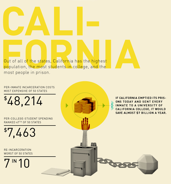
The only part of this graphic I kind of liked was the part about California. Here, we are able to compare the average cost of education for a year with the average cost of prison for a year. This is better than comparing the cost of a single school to the average cost of prison, especially when that school is as expensive as Princeton. I still have a problem with this comparison because the cost of school is running over about 8 months whereas the cost of prison is running the full 12 months, or at least that seems to be true from what I can gather. My back-of-the-envelope math suggests prison would be about $32,143 for 8 months. This is still much higher than the average of $7,463 per student spending for 8 months of school. Parent and student contributions to schooling are not factored in, though the point of the graphic is to compare what the state spends on students to what it spends on prisoners, ignoring the total amount spent on students.

What needs work

The information included in this graphic could have been presented in about one fifth of the space. I support the addition of graphical elements to information presentation only when they increase the clarity of the information provided or make the information delivery inarguably more elegant.

What I vastly dislike are the long columns of graphics stacked on top of each other, meant to be viewed as some kind of visual essay. That was where I drew the California graphic from. I pasted it below.

I’m curious. Do other people like these long, internet-only graphic essays? I find them extremely hard to digest. They seem to be plagued by apples-to-oranges faux comparisons, and unbashedly so. A year’s tuition at Princeton doesn’t include room and board. Prison does. Even if that were taken into account, the time frame is off.

One more item to highlight

Note that in the last panel they clue us into an uncomfortable reality: recent college graduates have a higher unemployment rate (12%) than the general population (9%). Ouch.

Prison vs. Princeton | Public Administration

References

Public Administration. (October 2011) “Prison vs. Princeton” [information graphic]

Resnick, Brian. (1 November 2011) Chart: One year of prison costs more than Princeton The Atlantic online.

Greenhouse gas emissions graph
Greenhouse gas emissions | World Resource Institue and Google's Public Data Explorer

What works

The World Resource Institute has partnered with Google to create an interactive portal for creating visualizations based on publicly available data. Google has been in the business of doing this sort of thing at least since the time they acquired Trendalyzer from Scottish-based gapminder.org in 2007. To be sure, gapminder.org is still a going concern of its own and IBM also offers free web-based visualization services through their Many Eyes program.

The focus of the trendalyzer is to show change over time and they succeed in making it quite easy to watch panel data change over time.

What needs work

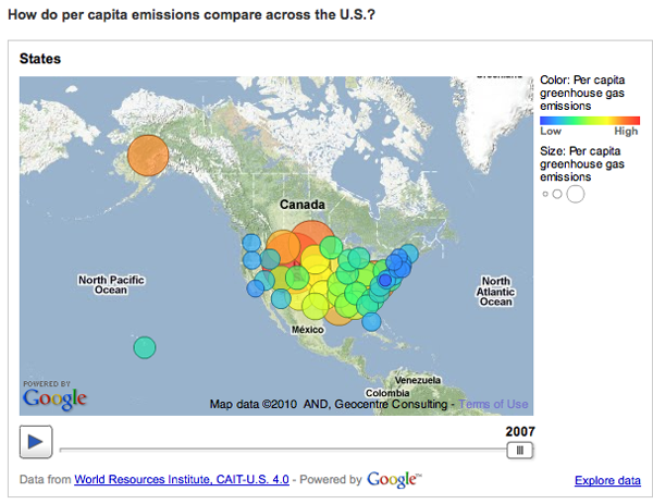
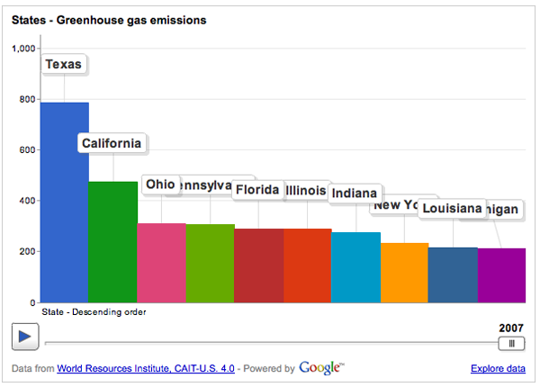
BUT…I find that this particular graphic is a great example of a misleading reliance on time as the key ‘context’ variable. So the graphic above breaks down greenhouse gas emissions by US state over the course of the year. If you have already clicked over to the World Resource Institute and watched the animation of these bars pumping up and down (more up than down) and trading places with each other over time, you will surely have been fascinated. I watched it three times in a row. But I was stuck wondering what the take away was meant to be. Clearly, there is the first order take away that the bars pretty much grow over time, they do not shrink. If I were the World Resource Institute, getting that message out would be important to me. But I would hope for more than just the bullhorn approach, “More is BAD! More is BAD!” which is kind of how this hits me at the moment.

One of the biggest problems with this graphic is: not all US states are the same size. Of course Texas emits more greenhouse gases than most states – many more people live there than in, say, Kentucky, Iowa, Oregon, etc. But the World Resource Institute chose to display per capita emissions with the bubble approach (which has almost no redeeming value in my opinion because I cannot even see half of the bubbles. Maybe they all could have been reduced by half or more? And maybe instead of going with colors on a spectrum, the worst could have been red, the best could have been green, and most everyone else could have been some shade of grey? It’s just not possible to hold 50 changing variables in your active cognitive space at once. Reducing it to three variables – the good, the bad and the mediocre – could actually increase retention and pattern recognition.)

Greenhouse Gas Emissions Per Capita, US 2007
Greenhouse Gas Emissions Per Capita, US 2007 | World Resource Institute and Google

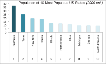
But back to the bar graph at the top. For the purposes of greenhouse gas emissions, it makes the most sense to interpret size as population not square miles, so that’s what I am going to do. In an attempt to be helpful, I threw together a bar graph of the top 10 most populous US states (using 2009 population estimates) in good old Excel. Note that our friend Texas is not the most populous state by about 12 million people – that is a lot of people. California is the biggest and they emit way less than Texas. New York is the third most populous state and we emit far less than our proportional share would suggest. Let’s hope it stays that way because I already find it unpleasant to breathe the air in Manhattan (admittedly, that could be due to many causes besides greenhouse gas emissions).

Most populous US states by size

My suggestion here is clear: prepare a bar graph per state, per capita. And, yes, I would want to see how that changes over time. I would probably watch the animation six times instead of three times. My fantasy is that we could compare not necessarily by state, because that is in many ways arbitrary, but by personal habits. Say we get the most extreme environmentalists – vegan, freegan, won’t even take motorized public transportation, never flies, prefers candles to compact fluorescents, has a composting toilet – to the somewhat average person who has a car but not an SUV, eats meat but not every day, does not pay more for organic food – to the extreme non-environmentalist who owns three houses, drives in an Escalade or something of that nature, flies internationally at least four times a year, pays extra for organic food (but at restaurants), and sends clothes to the dry cleaners twice a week. But that would probably result in a graphic best described as “info-porn”, enticing and exciting but intellectually vacuous.

Summary

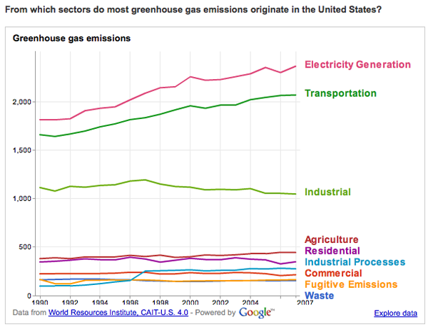
The WRI is on to something with their Google partnership. My favorite of their early work is this line graph that does a better job of telling the emissions story than any data broken down by state.

greenhouse gas origins
Greenhouse Gas Origins | World Resource Institute and Google

But the other great thing about the new partnership is that they ask for suggestions and set up a google group to manage the roll-out and incorporate nay-sayers like myself.

“By pairing [the Climate Analysis Indicators Tool] CAIT data with Google’s tools, there are new possibilities for people everywhere to take part in using sound data to tell stories that frame environmental problems and solutions. In the future, we hope to include additional data sets that can tell even more stories through Google’s visualization tools.

Suggestions for what you would like to see, or have a question about CAIT-U.S. data? Let us know here or join the conversation at http://groups.google.com/group/climate-analysis-indicators-tool.”

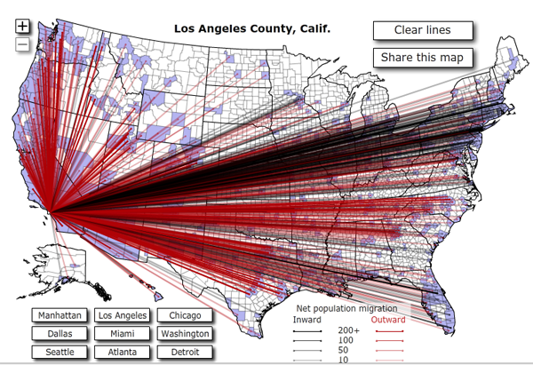
Migration into and out of Los Angeles, CA (2008)

What works

This is an interactive graphic situation so to get the most out of it, I recommend clicking through to forbes.com and playing around.

What works is that we can see a lot of internal migration between Los Angeles and other west coast cities as well as between LA, Florida, and the DC-NYC-Boston corridor. I know plenty of bi-coastal folks so the picture matches up with my experience. To get the proper context, I suggest you click through and pick some rural counties to see how much people tend to move from small place to small place and from big place to big place but not so much from very small to very big or vice versa.

Overall, what the interactive graphic ends up showing us is that people move quite a bit. The map gets saturated with lines.

Man, we can really make some cool graphics – and interactive ones at that – with the ridiculous capacity of desktop computers these days. This is a data-driven graphic that would have been nearly impossible not that long ago.

What needs work

There is no comparison for this graphic. I can’t tell if all this migration is more than normal, trending up, trending down, or anything of that nature. Sheer volume at one time can generate lots of questions but it doesn’t answer many.

I’d also be curious to know if the movers are evenly spread across the life course. Plenty of people move to go to college and then again when they leave college, or so I think. And there has been plenty of ink spilled about retirees moving south from places like Chicago and Minneapolis. Then, about ten years ago, I remember reading stories about the plight of the managerial class having to move around within their multi-national corporations to keep progressing in their companies all through their mid-life. With all those half-baked hypotheses, I would love to see how life stage impacts internal migration.

References

Bruner, Joseph. (15 June 2010) Map: Where Americans Are Moving at forbes.com.

Michael Schwabs poster design for the Art Center College of Design in Pasadena, CA

How to go from inspiration to design?

There are plenty of great graphic designers plastering walls with posters, filling magazines with intelligent ads, and even getting their work into museums. A lot of the time, it’s hard to see how all the inspiration and excitement of graphic design for advertising can make it’s way into the information graphics social scientists use to communicate their findings.

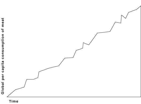
I took a fake example to show you how I translated my appreciation for Schwab’s design into some thoughts about enlivening a basic line graph. Let me emphasize this one more time: this example is fake. I didn’t use real data. Yes, global consumption of meat is increasing per capita, but no, it’s not as dramatic at it appears here. I went ahead and left off scales on the X and Y axes to ensure this graphic doesn’t end up traveling around the interwebs as truth.

Step 1

Break down Schwab’s graphic. He’s basically got a right triangle sitting on a single color background that bleeds into a thick border. The border contains the only text. The only realist element – the pencil – intersects the triangle to make what is like a giant X in the center of the poster.

How is this at all like social science graphics? Well, if you flip the triangle, it’s a lot like any positive relationship as depicted by a line graph.

Basic positive relationship depicted by a line graph

What next?

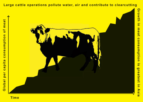
Now that you can see how a line graph is a little like Michael Schwab’s elegant pencil poster we can start to apply his decisions directly to our graphic. First, we can add a clearer background. If it’s just white the thick borders do not read as thick borders. They just look like the same old place everyone puts their axial labels. I distinguish this by adding a background color which will pull the borders into a relationship with the background behind the graph. I also go ahead and fill in the area under the graph to help nudge it into reading as an area, rather than some jiggly line.

The tough part here is the graphic. Not all stories we want to tell are going to be linked to a slender X-making image. I chose to depict the rise in meat consumption. Sure, I could have picked a cattle prod or other cattle killing tool dripping with blood. It would have been slender and I could have made an X. But I was trying not to appear unbiased so I just went with an iconic image of a beef cow. I planted the cow in the middle. We do lose a few data points in the middle – there are ways to deal with that if it’s important (overlay a yellow line across our cow’s gut where the data points are missing).

Here’s what we’ve got. The point is that the graphic below is the basically the same data as our line graph above except far more arresting (I took the liberty of adding two more lines of text – not necessary, but I was trying to closely follow Schwab’s concept). If you are trying to keep the attention of the audience in a presentation, be they sleepy students or sleepy colleagues, it might be worth your while to take a little extra time on your most important graphics. And if you do have one or two major points you want the people to take away from the graphic, you can write them across the top or up the side. Writing up the side is not as good – use it only for secondary points or graphic credits in the case that you hire someone to craft your graphics.

Simple line graph copying Michael Schwab's concept

References

Schwab, Michael. (2009) “Instrument of Creativity” [poster design] Art Center College of Design in Pasadena, CA.

Hirasuna, Delphine. (2009) “Art Center’s Instrument of Creativity” in At Issue Journal: The Online Journal of Business and Design. San Francisco, CA.

Cabspotting - San Francisco

What Works

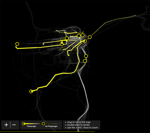
First, the elegant sophistication of this graphic is breathtaking. I love watching it and I have watched it for long enough to start asking questions about it. Maybe I am different than other people, an outlier of some sort, but in this case I don’t think so and that’s why my own fascination indicates a larger virtue of the graphic. If it draws people in and gets them asking questions, it is doing something right. Holding eyeballs in this media saturated world is a triumph in itself. Having answers to the questions that are posed is a secondary but even more critical step. To figure out what you’re looking at, here’s what the folks who made it have to say for themselves: “Cabspotting traces San Francisco’s taxi cabs as they travel throughout the Bay Area. The patterns traced by each cab create a living and always-changing map of city life. This map hints at economic, social, and cultural trends that are otherwise invisible. The Exploratorium has invited artists and researchers to use this information to reveal these “Invisible Dynamics.” The core of this project is the Cab Tracker. The Tracker averages the last four hours of cab routes into a ghostly image, and then draws the routes of ten in-progress cab rides over it.”

Second, they are right that just knowing where cabs go is more than knowing where cabs go. It’s knowing about urban space over time. It’s certainly knowing where the airport is (and that airports are far away). Looking at this we get to see the grid of the city and the longer stretch of highways and bridges bringing people in/out. It would be nice to see what this sort of ghostly cab mapping technique would reveal about cities I know a little better than San Francisco. Keep this site tucked in your back pocket for later this year, all you ASA meeting-goers.

What Needs Work

I just wish there were a simple way to say a little more about the cabbies themselves, who end up looking like infrastructure or phantoms, rather than actual people. In New York, 91% of the cab drivers are immigrants and only 1% are women (2006 Schaller Consulting). Is there a way that this cab-tracker could become a little more about the humans in the city?

Relevant Resources

Richards, P. and Schwartzenberg S. Snibbe S. and Balkin A. cabspotting San Francisco.

Schaller Consulting. Repository of Reports on Cabs in New York and beyond

Plaut, M. (2007) Hack: How I Stopped Worrying About What to do with my life and started driving a yellow cab. New York: Random House.

Buddhacab blog written by a New York yellow cab driver

Marijuana Arrests in New York City 1977 - 2006 (Harry G. Levine)

What Works

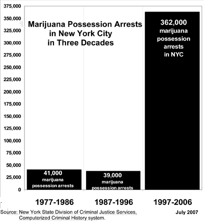
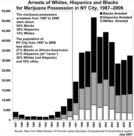
Sometimes simple is powerful. Everything here is well-labeled, the time periods move in even intervals and the source is cited. The point that arrests for marijuana possession have skyrocketed comes across almost instantly.

The graphic is taken from testimony given by Harry G. Levine, Professor of Sociology at Queens College and the CUNY-Grad Center to the New York State Assembly on Codes and Corrections:

“New York City has arrested about 100 mostly young people a day, every day, for the last ten years. By the end of today another 90 to 100 will be arrested. About 85% of the people arrested are Black or Latino, most are working class or poor, from the outer boroughs and from less affluent and poorer neighborhoods.”

Marijuana Arrests in New York 1987-2006 | Whites, Blacks, Hispanics

What Works

Levine includes this graphic in his testimony to demonstrate the uneven distribution of all these marijuana possession arrests across racial/ethnic boundaries. He is right to make sure to include a little decoder text about the distribution of whites, blacks, and hispanics as percentages of population of New York overall. Remember that in a world of equal arrest rates, whites would be arrested for possession roughly according to their percentage of the population, which is 36% in New York during the 1987-2006 period. But they were only accounted for 14% of the possession arrests. On the other hand, blacks should have been arrested 27% of the time but instead were arrested 54% of the time. Hispanics were the closest to even, representing 27% of the total population and 30% of the possession arrests.

What Needs Work

These stacked bar graphs always confuse people. So here we can use the y-axis to determine absolute number of arrests by racial/ethnic group but in other uses of this technique I’ve seen the bars all add to 100% and the viewer is supposed to suss out the relative proportion of the bar dedicated to the categorical break down. That clearly is not how this graph works, but still, where there is any chance of confusion, more work needs to be done to clear things up. I might have tried a hint of 3D, popping the white bar in front of the grey bar and the grey bar in front of the black bar just so that each bar reads as a distinct entity.

I would also have stuck the arrestee percentages directly next to the population percents. It would look more like:

Arrestees          Population
Blacks     54%     27%
Hispanics 30%     27%
Whites     14%     36%

Simple to do. Makes much more sense to read that data across rows. I would then have stuck the color shading key to the left of that little table and cut the “blacks arrested”, “whites arrested”, and “hispanics arrested” labels which would have cut down on the total amount of text the viewer would have to read through.

Go ahead and click through to the full report to see the other graphics and read the whole story about the astronomical increase in marijuana possession arrests in NYC with the disappointing follow-on that the arrests are being doled out in minority communities disproportionately more often than elsewhere in the city.

One parting quote to provoke you to jump across and read it all, in response to why there are so many arrests so unevenly distributed across the city’s population, “it is not because of any dramatic increase in marijuana use – which has not changed significantly since the early 1980s. Nor is the dramatic racial imbalance in the arrests the result of marijuana use patterns. In fact, marijuana use among Blacks and Hispanics is lower than for Whites, and has been for decades, as U.S. government statistics show. “

One More Thing

If you’re wondering where all the weed comes from, as I was, you might want to link through to the 2007 article “Home Grown” in The Economist via Proquest (subscription required) which notes in classically dry Economist fashion, “Marijuana is now by far California’s most valuable agricultural crop. Assuming, very optimistically, that the cops are finding every other plant, it is worth even more than the state’s famous wine industry.”

Relevant Resources

Becker, Howard. (1953) On Becoming a Marihuana User originally in American Journal of Sociology Vol. 59 November 1953 (235-242).

Dwyer, Jim. (30 April 2008) On Arrests, Demographics, and Marijuana The New York Times, NY/Region Section.

Levine, Harry G. (May 2007) Testimony before the New York State Assembly Committees on Codes and Assemblies.

Schlosser, Eric. (2003) Reefer Madness: Sex, Drugs and Cheap Labor in the American Black Market. First Mariner Books.

Home Grown: Cannabis in California (20 October 2007) in The Economist Vol. 385, Issue 8551 (60).

Piled Higher and Deeper - PhD Humor

What Works

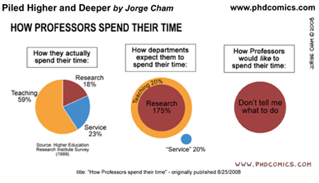
Humor is a slippery animal, indeed. I like to think of it as the pinnacle of culture, not in a high culture kind of way, but in a cultural development kind of way. Just think of trying to learn a foreign language. When you can intentionally, subtly be humorous in that language, you know you’re really getting somewhere. If you have never gotten to that point in a foreign language, just listen to kids try to tell jokes. They kind of suck. You end up laughing along because they’re kids and kids telling jokes is funny in itself, not because what they are saying is actually humorous. This is a fairly long winded way to point out that one indicator that telling stories with graphics is thick culture (thanks, Geertz) is that things like the above image are actually funny in a way that they couldn’t be funny in another format. If you had to say to someone, “man, professors spend lots of time on service activities, but the administration really doesn’t reward that or even notice” nobody would laugh. They might sigh and wish the economy were better so they could find a job that didn’t involve sitting on committees.

Bottom line: this works because we have been immersed in graphic storytelling. We get it. It doesn’t work in any other format.

Relevant Resources

Piled Higher and Deeper, a comic strip by Jorge Cham online. If you are a student or professor and haven’t discovered this, I’ll warn you that it could suck away an hour or two of your day if you click through right now.

Higher Education Research Institute at UCLA. The HERI Faculty Survey. There are fees associated with accessing the data but you can get an overview of how data about faculty time commitments is gathered.

This 2006 Obituary of Clifford Geertz in the New York Times does a good job of summarizing his life and work, for those who want to follow up on my parenthetical. His book “The Interpretation of Cultures” is a good place to start. If you want something shorter than a book, “Deep Play: Notes on a Balinese Cockfight” is worth a read.

<a href=
New Jersey Commission on Rationalizing Health Care Resources
Hospital Pricing Graph - SF Bay Area originally published in Health Affairs by Uwe Reinhardt

What Works

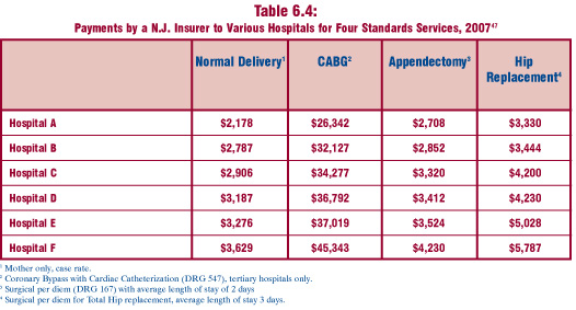
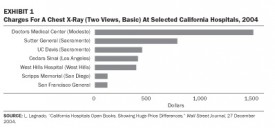
This comparison is a fairly straightforward examination of the relative merits of tables vs. charts.  Both of these images are trying to help explain the tricky business of health care pricing.  The bar graph comes from an article in Health Affairs by Uwe Reinhardt that starts by taking a look at the cost of a single procedure across hospitals within a small sample of hospitals in the state of California.  The table does the same sort of thing but it was written by the New Jersey Commission on Rationalizing Health Care Resources so it looks at hospitals in New Jersey.  It also looks across a number of treatments, not just one.

Each of these presentation styles has its merits.  The graph is an instantly legible message:  the cost of a chest X-ray varies a lot from one hospital to the next.  The table doesn’t have the same instant legibility but it provides much more detail across a range of treatments, demonstrating that the pattern of discrepant charges is not restricted to a single treatment.  Further, the table demonstrates a pattern – the relative cost of hospital treatments is fairly stable.  If a hospital charges at the low end for one treatment, it probably charges at the low end for all treatments.

What Needs Work

The bar graph does a good job of providing instant legibility but it doesn’t give much detail.  It works in the introduction of the paper to orient the reader but would not be nearly as useful in the results section because it shows only one treatment.

The table provides a lot of detail, but unless someone is already deeply interested in the problem of health care costs, they may not take the time to read it. No patterns are immediately obvious – it’s just a boxy sea of numbers. The presentation of the table as a graphic does little to help the eye.  At least the columns are arranged from lowest payment to the greatest payment.  They might have been made more visually legible if the font increased or the boxes got progressively darker as payment values increased down the columns.

Relevant Links

Chaos Behind a Veil of Secrecy in Health Affairs by Uwe E. Reinhardt

How Do Hospitals Get Paid – A Primer” on Nytimes.com Economix blog  by Uwe E. Reinhardt

New Jersey Commission on Rationalizing Health Care Resources, Final Report 2008 by the State of New Jersey Department of Health and Senior Services