methods/use of data

Greg Mankiw, a big shot economist (he was the chairman of President Bush’s Council of Economic Advisors) had a brief blog post on Monday comparing European countries and the US. It’s part of a long-standing debate about the relative merits of European-style social democracy. The left wants the US goverment to do more to reduce inequalities (ensuring universal health care, for example, or providing benefits for the unemployed, and the poor, requiring employers to offer paid maternity leave, etc.). Those on the right argue that these policies would stifle the economy. They offer an economic picture of America the dynamic, Europe the stagnant.

The volume on that debate got turned up by an article by Jim Manzi in National Affairs. He refers to “government policies — to reduce inequality or ensure access to jobs, education, housing, or health care — that can in turn undercut growth and prosperity.”

Paul Krugman, in his column on Monday, rejected this idea:

The real lesson from Europe is actually the opposite of what conservatives claim: Europe is an economic success, and that success shows that social democracy works.

Greg Mankiw gives some data on GDP per capita, adding with a sly grin, “Readers of today’s column by Paul Krugman might find these figures useful to keep in mind.” He gives the data for “the United States and the five most populous countries in Western Europe.”

We’re number one. We’re way ahead – 30% higher than the UK next in line. Mankiw wins; Krugman loses. Case closed. Or is it?

I’m sure there’s a good economic reason for this cherry-picking choosing only the five largest cherries. But if you were curious about some of the insignificant countries in Europe and elsewhere, you might want to take a look at the entire list. Here’s an expanded chart:

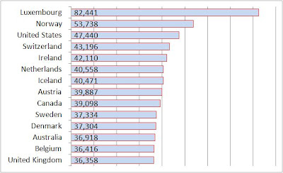
It turns out that among the non-Asian industrial democracies, there are a few countries that fall in that $11,000 gap between the US and UK. And when you include all those countries, the US is no longer number one.

Please welcome Guest Blogger Philip Cohen.  Cohen is a sociology professor at the University of North Carolina at Chapel Hill where he specializes in studying the family.  We are pleased to reproduce a post from his own blog, Family Inequality, about (how statistics lie and) the recent media hype about the decrease in the divorce rate.

—————————————-

Delivering some “good news for Christmas,” The National Marriage Project, under the editorship of the sociologist W. Bradford Wilcox, has released a report titled The State of Our Unions, 2009: Money and Marriage. It has a lot of useful information on marriage and families, with some editorial bending in the pro-marriage-and-family direction.

My beef here is with the chapter titled “The Great Recession’s Silver Lining?” In it, Wilcox writes:

judging by divorce trends, many couples appear to be developing a new appreciation for the economic and social support that marriage can provide in tough times. Thus, one piece of good news emerging from the last two years is that marital stability is up.

That line was quoted by Ross Douthat at the New York Times, which is a shame, because there is no evidence about anyone’s appreciation for marriage in the chapter. Instead, the evidence for this assertion is presented in a graph that shows three data points in the divorce-rate trend:

The figure shows a decline in the divorce rate from 2007 to 2008. In the press release he calls that drop “the first annual dip since 2005.” (The rate shown here is divorces in a given year per 1,000 married women in the population that year.) Couple things:

1. There is no data point for 2006, so for all we know the divorce rate actually rose higher than it was in 2007, and started falling before the recession, which officially began in December 2007.

2. Despite the dramatic turnaround apparent in this graph, it’s really not enough to go on to draw the kind of conclusion he draws.

The second point is more important, because there really is a lot of research that shows job loss increases the odds of divorce. So why should this recession be different? It’s possible it is, but there’s no evidence – in this report or elsewhere that I’ve seen – of such a change.

In fairness, Wilcox wrote a column in the Wall Street Journal that musters some anecdotal evidence for his theory. But nothing to get him this far: “For most married Americans, the Great Recession seems to be solidifying, not eroding, the marital bond.” Even if the divorce did drop a little in one year – that doesn’t say anything about “most married Americans.”

That three-point graph is especially unfortunate because it leads to interpretations like this: “The divorce rate … had previously been on an upward path, rising from 16.4 divorces per 1,000 married women in 2005 to 17.5 in 2007.” That seriously misstates the real trend in divorce rates, which have actually been falling since 1981. And there is nothing in the trend to suggest that recessions teach couples a “new appreciation for the economic and social support that marriage can provide in tough times.” In the appendix, Wilcox presents that longer trend, which makes his previous figure seem much less dramatic.

(The graph seems a little off to me – notice how 10.6 is closer to the line for 10 than 14.9 is to the line for 15 – but I’ll work from his numbers below anyway.)

I think the story of a turnaround in divorce rates has traction because, like crime, divorce is one of those things many people assume is always getting worse (I see this in student papers frequently). So any decline in divorce rates looks like an important change.

What is recession’s effect?

I previously speculated that, because this recession was costing so many men their jobs, more men were likely to be become primary caregivers, and do more housework. The downside – I speculated – was that “maybe men getting ’stuck’ with childcare doesn’t bode well for marriages.” To support that speculation, I showed a graph of divorce rates that had little upward spikes during some recent recessions. The graph was not the real evidence for the argument – which was here:

We already know that economic hard times contribute to marital instability and divorce. Studyafter study after study have found that losing a job increases the likelihood of divorce, with some evidence that husbands’ losses matter more.

Here is a new graph I made, with the “crude divorce rate” (divorces per 1,000 people in the population) in blue, superimposed over Wilcox’s calculations in red. (His takes more work, which is probably why he doesn’t have it for every year. But they track quite well, with some pulling apart some after 1980, which has to do with changes in the population composition that probably aren’t important.) I also put the recessions on there, roughly, by hand with purple bars.

Source: Divorce rates from 2010 Statistical Abstract and various prior years; business cycles from 2010 Statistical Abstract.

Two things here:

1. Over the longer run, there is no obvious relationship between recessions and the divorce rate. There are big social forces at work here (like the rise of the legal practice of no-fault divorce, the increase in women’s education and employment, the growing tendency of men and women of similar education levels to marry, later age at marriage, more cohabitation and unmarried childbearing, etc.). But on the surface – which is where the Wilcox conclusion is drawn – there is not much to go on.

2. The crude divorce rate I got from the Statistical Abstracts shows a little peak in 2006 – not 2007 – followed by two consecutive years of decline, beginning before the recession. So rather than talk about the reason for the decline in the last year – which really just fits in with the falling divorce rates since 1981 – the anomaly is 2006. I have no explanation for that, but in the long run it probably doesn’t matter much.

On the other hand, the American Academy of Matrimonial Lawyers has surveyed its members twice since the recession started. In the first release last fall, they said 37% expected a drop in divorce filings, compared with 19% who usually see an increase during recessions. This fall they report that 57% of their members experienced a drop in filings, with just 14% seeing an increase. There are no details or methods reported in these releases, so it’s hard to evaluate. But if it’s true – along with the previous evidence that unemployment increases divorce – then it maybe that recessions delay the timing of divorce filings while increasing the divorce rate for those affected in the long run.

On the third hand, Jay Livingston at Montclair State points out that the NY Times reports that, in New York’s recession-year court backlog,  ”Cases involving charges like assault by family members were up 18 percent statewide.”

Whether delayed divorce filings contribute to family violence is a question someone might be able to answer when they put all this together. But I doubt the final word will end up as simple as, “Couples too broke to bicker,” as heartwarming as that is. There may be something to the speculation that falling home prices are stalling some divorce plans, but that is not quite the same as developing a newfound appreciation for the benefits of marriage.

I’m sticking with this: in hard times, families are a big part of how people make it through, but hard times are also hard for a lot of marriages. If it’s true that the husband’s job loss especially increases stress on a marriage – as previous research suggests – we may yet see that emerge for the current crisis. If not, maybe something has changed.

Lisa Wade, PhD is an Associate Professor at Tulane University. She is the author of American Hookup, a book about college sexual culture; a textbook about gender; and a forthcoming introductory text: Terrible Magnificent Sociology. You can follow her on Twitter and Instagram.

An anonymous confession sent to PostSecret, a site for secrets:

See also our post on the plagiarized dissertation of then-Jacksonville State University president, William Meehan.

Lisa Wade, PhD is an Associate Professor at Tulane University. She is the author of American Hookup, a book about college sexual culture; a textbook about gender; and a forthcoming introductory text: Terrible Magnificent Sociology. You can follow her on Twitter and Instagram.

OKCupid, an online matchmaking site, offers data on gender and perceived attractiveness that I might use in my spring deviance course (via boing). The figures might help me make a Durkheimian society of (hot) saints point about the relative nature of beauty and a Goffman point on stigma affecting social interaction, while providing another illustration of the taken-for-grantedness of heteronormativity.

In any case, the first figure shows that male OKCupid ratings of female OKCupid users follows something like a normal distribution, with mean=2.5 on a 0-to-5 scale from “least attractive” to “most attractive.” Also, women rated as more attractive tend to get more messages. At first, I thought I saw evidence of positive deviance here, since women rated as most attractive get fewer messages than those rated somewhat below them — the 4.5s garner more attention than the 5.0s. But, as I’ll show below with the next chart, that would probably be an incorrect interpretation — confounding the “persons” in the dashed lines with the “messages” in the solid lines.

The next figure shows that female OKCupid users tend to rate most male OKCupid users as well below “medium” in attractiveness. According to OKCupid, “women rate an incredible 80% of guys as worse-looking than medium. Very harsh. On the other hand, when it comes to actual messaging, women shift their expectations only just slightly ahead of the curve, which is a healthier pattern than guys’ pursuing the all-but-unattainable.”

Hmm. The latter point isn’t wrong, I guess, but it shouldn’t obscure the bigger point that more attractive men still get more messages than less attractive men. Again, note that persons (OKCupid members) are the units of analysis for the dashed lines and messages (messages sent by OKCupid members) are the units for the solid lines. On first scan, I read the graph as suggesting that the top “attractiveness quintile” was getting fewer messages than the bottom attractiveness quintile — that uglier men were actually doing better than more attractive men — but that’s not the case at all. Instead, it just means that in the land of the hideous, the somewhat-less-than-loathsome man is king.

If almost everybody is rated as unattractive, most of the messages will go to those rated as unattractive. Nevertheless, the rate of messages-per-person still rises monotonically with attractiveness. As the “message multiplier” chart below shows, the most attractive men get about 11 times the messages of the least attractive men — and the most attractive women get about 25 times the messages of the least attractive women.

—————————

Chris Uggen is Distinguished McKnight Professor and Chair of Sociology at the University of Minnesota.  His writing appears in American Sociological Review, American Journal of Sociology, Criminology, and Law & Society Review and in media such as the New York Times, The Economist, and NPR.  With Jeff Manza, he wrote Locked Out: Felon Disenfranchisement and American Democracy.

If you would like to write a post for Sociological Images, please see our Guidelines for Guest Bloggers.

At least it is according to words referencing happy and unhappy states in our Facebook status updates:

It’s probably just an artifact of people using the word “grateful” because they’re supposed to.  Then again, maybe being reminded to be grateful really does make people happy for a day.

Source: Facebook via Flowing Data.

—————————

Lisa Wade is a professor of sociology at Occidental College. You can follow her on Twitter and Facebook.

This last week New York Times suggesting that older woman/younger man relationships were on the rise.  But I wouldn’t get too excited just yet.  The data below shows that the percentage of men marrying women ten and especially five years younger is decreasing and the percentage of women marrying men ten and especially five years younger is increasing.

It all looks very dramatic until you check out the y axis.  Notice that the y axis for the “husband older” graph is zero to 35%, but the y axis for the “wife older” graph is zero to 10%.  This makes the data for men look more impressive than it is.  Not that 8 or 10 percentage points is insignificant, but it would be far less impressive on a zero to 100 scale.  The data for the women, especially sitting right next to the “husband older” table, look far more impressive than it is.

Only about 6% of women are marrying men five years younger or more.  That’s a two percentage point increase since 1960.  Not exactly a cougar revolution.  One in four men are still marrying women five years younger or more.  And, though it appears that they’re not marrying women five years younger or more as frequently, the age distribution of the remaining 69% of marriages is left invisible and most of them probably involve women that are somewhat younger than their husbands.

So, yes, today women are more likely to marry younger men than they were in 1960.  But the presentation of the data (the inconsistency in the y axis) makes the degree of difference seem larger than it is.

—————————

Lisa Wade is a professor of sociology at Occidental College. You can follow her on Twitter and Facebook.

In the Bible (book of Genesis), God sends two angels to the cities of Sodom and Gomorrah. These angels were charged with the task of evaluating the rate of sin within the walls. If the people were completely overridden by sin, God would destroy them.

What if those angels were statisticians, with access to GIS and geomapping software? How would the story have been different?

Some geographers at Kansas State University recently did an analysis of the spacial distribution of EVIL in the United States. Which part of the country is most afflicted by sloth? Lust? Greed? Envy? Wrath? Gluttony? Pride?

That’s right, folks – these geographers have operationalized sin, quantified it, then measured and mapped it. Pride is the aggregate distribution of all other sins, since it is supposedly the root of all evil (though one could also make a good case for apathy). Here’s how the sins are measured (and here’s a good view of the maps):

• Greed: Average incomes versus total inhabitants below the poverty line
• Envy: Total number of thefts (robbery, burglary, larceny, and stolen cars)
• Wrath: Total number of violent crimes (murder, assault and rape) per capita
• Lust: Sexually transmitted diseases per capita
• Gluttony: Number of fast-foot restaurants per capita
• Sloth: Expenditures on arts, entertainment and recreation versus rate of employment
• Pride: An aggregate of the six other sins

By looking at sin at the aggregate level, what they’re doing here is examining sin as a social fact, as opposed to an individual trait. This would be a good extension of a lesson on Durkheim and suicide as a social fact. This study really shows why we really can’t truly measure concepts such as this across space and time, since the meaning of these individual acts will vary. Are the same acts categorized and labeled as rape in Montana as they are in New York? How violent does a person need to be before they are arrested for assault, and does that differ by region? Are we really measuring rates of STDs, or rates at which people get treatment for them? If my measure of gluttony is different than yours, can I apply my measure to your actions and call you gluttonous? Or should I be using your measures to evaluate your actions? Is this aggregate data showing different rates of sin, or is it just an effect of different meanings attached to the concepts?

This would also be useful in showing how we can’t extrapolate individual characteristics from aggregate data. For example, I live in Indiana (but teach in Kentucky). This region is low in envy, lust, wrath, and pride; average in gluttony, sloth, and greed; and not particularly high in any of the sins. Apparently I live in one of the more virtuous parts of the country.

I guess I can cancel that fire and brimstone insurance.

But does this aggregate data also indicate that I, Anomie, have greater odds of being virtuous? NO. The fact that I am virtuous in every way is merely a coincidence. You see, their data is not measuring individual sinful behavior. Rather, it’s measuring social facts, and structural conditions, that they hypothesize to be correlated with individual sinful behavior (but I take issue with some of the measures). For example:

• I don’t have any STDS. CLEARLY I am not lustful. CLEARLY.
• If you have more fast food restaurants within a five mile radius of your house than I do, are you more gluttonous than me? No. But at the aggregate level, this may be a good quick and dirty device. At least they didn’t use obesity rates as their measure.
• And if I make $100k (one can dream) in Indiana, then move elsewhere to a job with the same salary, does that mean my greediness has changed along with my place of residence?

Now, excuse me while I get back to my slothful appreciation of art.

——————————

Angie Andriot, also known as Wicked Anomie, maintains the (mostly) sociology blog Wicked Anomie: Sociology Run Amok. On occasion, she likes to toss off her cape, hop offline, and play the role of Angie Andriot: Grad Student Extraordinaire – deftly juggling the writing of her dazzling dissertation at Purdue University with the imparting of wisdom to her lovely students at University of Louisville. She is particularly fond of symbolic interactionism. And cheese.

If you would like to write a post for Sociological Images, please see our Guidelines for Guest Bloggers.

Using maternal mortality, Hans Rosling illustrates the uncertainty in different ways of measuring variables:

Found at GapMinder.

—————————

Lisa Wade is a professor of sociology at Occidental College. You can follow her on Twitter and Facebook.