demography

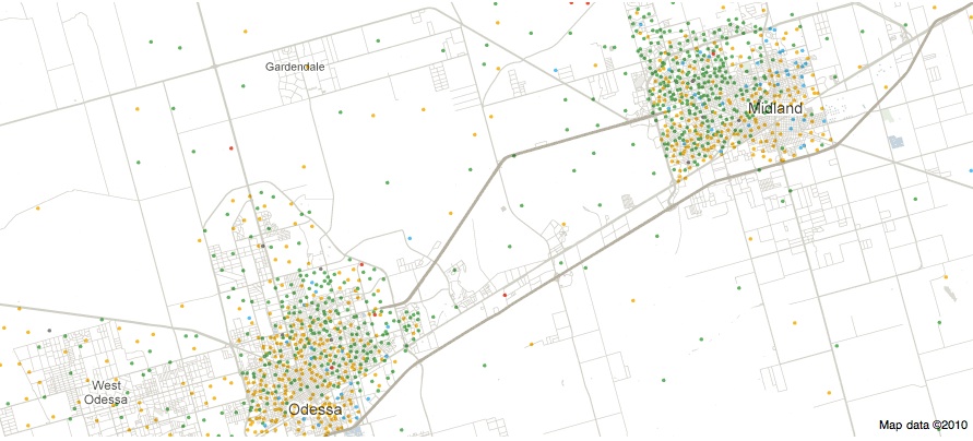
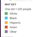
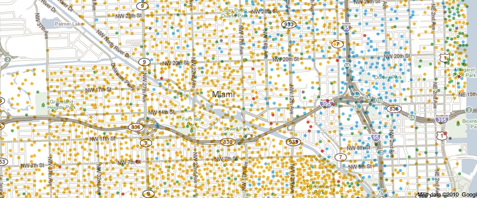
The U.S. Census Bureau has started releasing data from the 2010 Census. This map shows the change in the racial/ethnic minority (i.e., anything other than non-Hispanic White) population over the last decade:

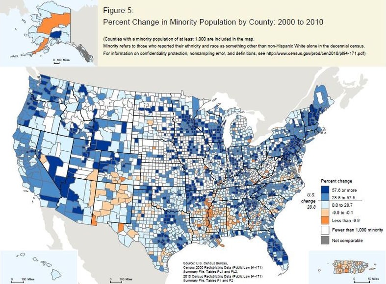
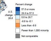
Legend:

They released a report, An Overview: Race and Hispanic Origin in the 2010 Census (available here), which includes data on those who reported more than one race. Among those who reported more than one race, the vast majority listed two. Here are the most commonly reported combinations:

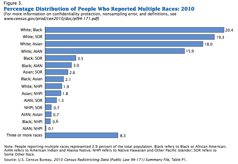
AIAN = American Indian/Alaska Native, NHPI = Native Hawaiian/Pacific Islander, and SOR = some other race.

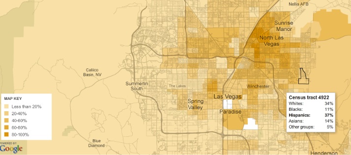
Laura E. pointed out that New Geography posted some maps based on 2010 Census data. Here’s the Hispanic population as a percent of the total population, by county (notice that the legend need to be multiplied by 100 to get the percent):

The African American population (alone or in combination with another race, and again, multiply by 100):

Thelittlepecan let us know that the World Health Organization has out a new report about global alcohol consumption, as well as the consequences of that consumption. Overall consumption varies significantly, with the highest levels in Russia and much of Europe and the lowest in northern Africa through Asia (the consumption figures exclude tourists):

There are also clear differences in the most-consumed type of alcoholic drinks:

The report also looks at what proportion of all male deaths are related to alcohol consumption, broken down by region, age, and sex. Globally, alcohol-related problems are the leading cause of death for males aged 15-59. For the regions, AFR = Africa, AMR = Americas, EMR = Eastern Mediterranean, EUR = Europe, SEAR = South East Asia, and WPR = Western Pacific:

Clearly the Americas and Europe stand out, though this is  likely because those regions have lower death rates from many sources that are still prevalent in many parts of the world and, thus, alcohol-related ones show up more prominently.

Differences in blood-alcohol limits for drivers:

If you’re interested in more details, you can also get profiles of individual countries in each region at the WHO website.

Well, it’s 2011. Sometime this year, the global population will pass the 7 billion mark. Jessica B. sent in this video, from National Geographic, that puts that into some perspective, showing the rapid increase in the pace of population growth over time:

Back in September, I posted about some maps put together by Eric Fischer, using 2000 Census data, showing the racial/ethnic makeup of selected cities. As Jeff H., Eluned J., and Dmitriy T.M. pointed out, the NYT now has up an interactive map where you can see the racial/ethnic composition of any Census tract, using more updated Census Bureau data from 2005 to 2009. For instance, here’s a map of the neighboring cities of Midland and Odessa, Texas, which I picked for no reason other than that I just watched an episode of Friday Night Lights, which is set in a fictionalized version:

Color key:

You can zoom in to get quite detailed information about individual neighborhoods. I zoomed in as far as I could on Miami (each dot now represents 50 people):

There’s also a tab that says “View More Maps.” It allows you to select to see just the distribution of Whites, Blacks, Hispanics, Asians, or the foreign-born population. Here’s the map of the Hispanic population of Las Vegas:

As you can see, if you hover over a Census tract, you can get specific data on its racial/ethnic makeup.

The foreign-born population of Seattle (if you hover over a tract, it will tell you the % foreign-born, as well as the % increase in the foreign-born population since 2000):

A great resource. Although I tried to look up my home town, and even zooming in to the smallest scale, it’s too small to have any data available.

The NYT has posted an interesting interactive map showing the results of the last slave Census taken in the U.S., in 1860, which I discovered via Jessica Brown and Jim Yocom. The map, which shows county-level data, illustrates how slave ownership varied throughout the South

The shading (a new technique at the time, according to the NYT article) indicates what percent of the entire county’s population was enslaved:

You can see the percentage for each county, which is listed on the map, more easily if you zoom in on the pdf version. The cotton-belt area along the Mississippi River clearly stands out, as does Beaufort County, South Carolina, all with over 80% of the population enslaved. The highest rate I could pick out (the map got a little blurry as I zoomed) is in Issaquena County, Mississippi, where slaves appear to have made up 92.5% of the population.

The map also included information on the overall population and % enslaved at the state level; in South Carolina and Mississippi, over half of the total state population was made up of slaves:

Also check out Lisa’s post on geology, the economy, and the concentration of slavery in the U.S.

As the NYT post points out, the map doesn’t show the dramatic increases in slavery in some areas. For instance, while Texas ranked fairly low in terms of the overall slave population, the number of slaves in the state had tripled between 1850 and 1860. The number had doubled in Mississippi between 1840 and 1860. Those growth rates make it rather hard to swallow the argument sometimes presented by those romanticizing the Confederacy that slavery was actually on the wane and would have soon been ended in the South anyway, without any need for federal interference, and wasn’t why the South seceded at all.

Jon Stewart and Larry Wilmore discussed this effort to frame discourses about the Civil War to erase the issue of slavery on The Daily Show:

Dmitriy T.M. sent in a video where Hans Rosling illustrates changes in wealth and life expectancy in 200 countries over the past 200 years, all in four minutes. Pretty neat!

Dmitriy T.M. and Jeff H. sent in a link to Mapping the Measure of America, a website by the Social Science Research Council that provides an amazing amount of information about various measures of economic/human development in the U.S. Here’s a map showing median personal (not household) earnings in 2009:

The District of Columbia has the highest, at $40,342; the lowest is Arkansas, at $23,470 (if you go to their website, you can scroll over the bars on the left and it will list each state and its median income, or you can hover over a state).

You can break the data down by race and sex as well. Here’s median personal income for Native American women, specifically (apparently there is only sufficient data to report for a few states):

Native American women’s highest median income, in Washington ($22,181), is  lower than the overall median income in Arkansas, which is the lowest in the U.S. as we saw above.

Here is the percent of children under age 6 who live below the poverty line (for all races):

Life expectancy at birth differs by nearly 7 years between the lowest — 74.81 years in Mississippi — to the highest — 81.48 years in Hawaii:

It’s significantly lower for African American men, however, with a life expectancy of only 66.22 years in D.C. (again, several states had insufficient data):

The site has more information than I could ever fully discuss here (including crime rates, various health indicators, all types of educational attainment measures, commuting time, political participation, sex of elected officials, environmental pollutants, and on and on), and it’s fairly addictive searching different topics, looking data up by zip code to get an overview of a particular area, and so on. Have fun!

My friend Captain Crab (happy late birthday!) pointed out a graphic at Portfolio that displays the results of their metropolitan “stress test,” in which they use ten measures such as poverty level, unemployment rate, commute, mortgage affordability, etc., to quantify how stressful different metro areas are to live in currently. Obviously it’s a rough measure — they usually use the rates of central cities rather than the larger metro area, people may interpret the same seemingly objective levels of negative or positive factors very differently in terms of how stressed they feel, only the 50 largest metro areas are included, and I don’t know if there’s clear evidence linking less-sunny places to less stress (anyone know?) — but it does provide a snapshot of how different cities compare.

You can hover over a city to get info on its ranking; since I live in Vegas, I checked it out, which has the highest unemployment rate of the 50 metro areas studied, but hey, we get lots of sun!

Just to clarify, the mortgage indicator isn’t the average mortgage, it’s the “affordability” of the mortgage “expressed as median house value per $1,000 of median household income”. The most unaffordable city? New York, followed by L.A.

The overall most stressful city is Detroit; the least is Salt Lake City. If you want to waste more time comparing the rankings on each of the ten measures, they have tables listing the results.