graphs

Mapping Singles - J. Soma

What Works

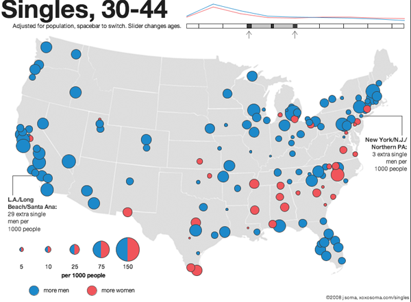
Your sense of who’s single and when they’re single will grow immensely in three or four minutes of playing around with this interactive map of single-ness in the United States, by age and gender. Men get married later and die younger. This means that at young ages, there are more single men than single women because some men who will eventually get married won’t marry until later, on average, than the women they end up marrying. This is just a complicated way of saying that men often marry younger women. In old age, there are more single women than men (the imbalance is because the men start dying younger). During the decade of the twenties and then after about age 65 you’ll find the largest proportions of single-ness. People in the middle decades, from 30-60 or so, are more likely to be coupled. But don’t take my word for it, click through and play around. This data actually understates the number of people who are functionally single because single is measured here as never married. So the folks who have been divorced or widowed and haven’t remarried do not count as single for the purposes of this graphic.

The writer of the text accompanying the graphic is interested in the geographical distribution of single women and single men so there’s more on that if you click through.

What Needs Work

I like this one a whole lot so I don’t have much to say except that I wish the designer wouldn’t have gone with the red/blue, female/male color scheme. How about purple and green? Or orange and teal?

I also think I would have counted people who are divorced/widowed and NOT remarried as single.

The graphic designer is careful to note that since homosexual couples cannot get married, they will erroneously be counted as single, even if they are partnered. That’s a problem with the underlying data collected by the census, not the graphic design.

Relevant Resources

American Community Survey (2006)

Soma, Jonathan. (2008) The Interactive Singles Map

Simple SIR model - Epidemic Spread

What Works

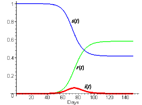
The relationship between infectious agents and the host populations is a tricky one, with three-parts at the very least. In order to understand how they relate, it helps to visualize what could otherwise be spelled out. In this graph, s(t) represents the proportion of the population who is susceptible (ie unexposed) to the infectious agent, r(t) represents the recovered population, and i(t) represents in the infected population – all are varying over time. You can see that everyone starts out susceptible, but slowly that proportion drops, though it doesn’t drop to zero. Some portions of the population are likely to remain uninfected. Note that the exact shape and inflection of these trend lines will depend on the particulars of the infectious agent – fatal agents have models that look different from non-fatal agents, long latency periods model differently than short latency periods.

Note the the peak of the i(t) trend will come before the crossover of the recovered and susceptible trends, as it does in this case. As soon as the derivative of the infection rate becomes negative, more people will have recovered than are susceptible and those two trend lines will intersect. I love this sort of graph.

What Needs Work

I would love this graph a whole lot more if it had a legend and applied to some specific disease. That’s mostly my fault.

Motorcycle Deaths vs. Car Death Rates

What Works

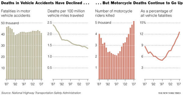
This story is a little dated – it was published when gas prices were at $4 a gallon. The facts, as written, look something like this: “Deaths on motorcycles hit a low of 2,116 in 1997. Since, they have risen 128 percent. Their share of crash fatalities has jumped to almost 13 percent from 5 percent.” In this graphic, we’ve got absolute numbers of fatalities by vehicle type in the bar graph and some sort of relative measure in the line graphs. I am not sure four graphs together is the most elegant way to show this information, but it does the trick. We see that car fatalities are trending downwards slightly while motorcycle fatalities are trending upwards. What we don’t see is that fewer cars were on the road and more motorcycles were out there. People shifted from gas guzzling cars to more efficient motorcycles or to public transportation. One would expect that with more motorcycles there would be more motorcycle accidents and that with fewer overall drivers there would be fewer car accidents. So how much of this is a real change in the relative danger of riding a motorcycle versus driving a car, which is what these graphs and the accompanying story are trying to suggest exists?

What Needs Work

I like that the absolute measures of car fatalities and motorcycle fatalities are directly comparable. I don’t like that they chose to look at two different relative measures. We’ve got deaths per 100 million miles driven for cars and motorcycle deaths as a percentage of all vehicle fatalities for our relative measures and that just doesn’t make for any kind of rational direct comparison. They are two completely different kinds of measures.

Note

Wear helmets. A mind is a terrible thing to waste, especially when it’s your own.

Relevant Resources

Wald, M. (2008, 14 August) Deaths of Motorcyclists Rise Again in The New York Times, US Section.

Cost of Transit - Derived from (1999) Transportation for Livable Cities By Vukan R. Vuchic

Reader Note

It’s been nice to be away at a couple of conferences and a few days alone in Paris, but now I’m back and so is Graphic Sociology. I thought I might come across more material to discuss here. Much to my dismay, I saw hardly anything by way of charts, diagrams, or graphics used to support/illustrate sociological arguments. Tomorrow I have something from the Corporation for Public Broadcasting courtesy of a panel at the Eastern Sociological Association, but that really is about all I’ve got so far.

What Works

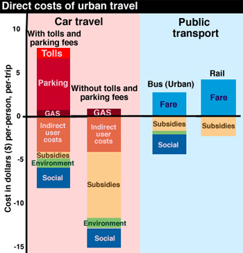
The above graphic is something I found on the interwebs though it was derived from a book that I admittedly have not read. With that in mind, I am not going to be able to comment on the veracity of the data. What I can comment on is the strategy employed to organize the information.

First, the use of color to split public transit from private car travel is quite helpful.

Second, I am pleased at the use of the zero line. The use of the zero line allows the graphic to establish a binary that quickly registers as a sort of good/bad moral binary. Often the zero line draws a distinction between good and bad where the good is growth and the bad is shrinkage (think financial graphics – they’re always sticking growth on the plus side of zero and shrinkage on the negative side). Values above the line mean one thing, things below the line mean a opposite, or at least directly opposed, worse thing. In this case, the good kind of transit expenditure is the expenditure that accrues to the individual and the amounts on the negative side of the zero line represent portions of transit that are paid for by larger collectives.

What Needs Work

I don’t understand the use of color beyond the blue/red division between public transit and car travel. It seems both arbitrary and not especially pleasing to my eye.

The category “environment” and “social” are not instantly legible but at least they’re better than “indirect user costs”. The use of precisely chosen language is critically important in graphics because it’s fairly easy to assume that many people are not going to read your text. Since I don’t have the book, I can’t even post the relevant text here to help clarify what those categories represent in detail.

My biggest concern with this graphic is one of the things I like about it: the use of the zero line. Generally speaking, using a zero line gives graphics greater dimensionality because of the greater symbolic value of zero compared to other numbers. In terms of absolute value, this graphic could have just showed us the net costs of transit options which then could have been represented as values where zero was a minimum value. In that depiction, rail would be the tallest bar and car travel without tolls and parking fees could have been set to equal zero. (what you would be looking at there would be the difference in cost between the modes of transit). Using the zero line here allows for a distinction between public and private expenditures on transit which is good.

BUT…the implication that the zero line divides the positive from the negative, the good from the bad, makes it look like public funding for transit is a bad thing while private expenditures are good. This is problematic. I can see what the author is trying to nudge us towards – that people who drive private cars pass a lot of the cost of that behavior on to collective populations. All the bus and subway riders are still breathing air polluted by passenger and delivery vehicles even as they spend more time out on the street walking to the subway and bus stop. However, this graph implies that all public funding or cost-bearing for transit is bad while private expenditures are good. This carries a decidedly pro-capitalist, up by your bootstraps kind of political implication. If you look closely, it isn’t that hard to see that imposing parking fees seems to decrease the amount of public subsidy to its lowest point.

I don’t know the overall message of the book where this graphic was derived but I imagine that it was pro-public transit. This graphic subtly disservices that message by indicating that all public expenditure on transit is bad. The strongest message I draw from this is that parking isn’t expensive enough and neither is gas. Also, that the social costs are incorrectly calculated – how can they be non-existent for rail and the same for cars with cheap parking, cars with expensive parking, and buses? Buses are louder and smellier than cars but I’m more likely to be killed by a car than a bus. Noise, smell and the potential for fatality seem to be social costs, but how can they be weighed against each other? Seems like a classic apples to oranges problem hidden in a little blue block. This is on top of the bigger problem that public subsidy is going to attend all transit options and is not necessarily a negative thing, neither is private payment for transit necessarily a positive thing. There are those who suggest that mobility should be considered a public good, something to which everyone should have equal access, thus private payment is necessarily a bad thing because it is regressive.

Flattening all the categories into the same kind of value – environmental costs are the same sort of thing as social and public subsidy costs – makes it possible to graph these things, but is troubling. Because I don’t know what is included in the environmental costs or how they are calculated, it’s hard for me to tell whether or not I would prefer to increase subsidies now (or increase fares and parking fees) to avoid environmental costs that could have significant long term consequences which will be even more costly in the future than they are at the moment. I mean, if the environmental costs include things like extremely high rates of asthma in poor communities that abut highways, I might think that’s too high a lifestyle price to pay even if the actual cost of treating the asthma is calculable and relatively low. (Maybe that “social” cost category includes things like monetizing lifestyles – what does a life riddled with asthma cost?)

Context

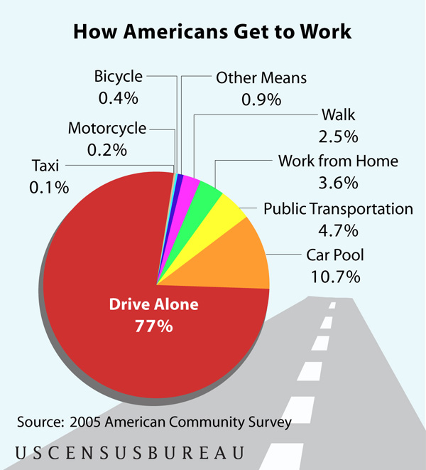
Just to contextualize this debate a little more, the following chart was derived from the American Community Survey of the US Census Bureau (2005) and shows just how people get to work. Commuting is the type of travel in which people are most likely to take public transportation – more so than taking one off trips to shop or visit friends and family. As you can see, public transit makes up a fairly small percentage of American’s transit behaviors. This is changing, public transit is experiencing growth in rider-ship, but chipping away at that three-quarters of the population whose experience of mobility is private and on-demand, is not going to happen overnight.

American Commute - Census Data

Relevant Resources

American Public Transportation Association

US Census Bureau. (2007 June 13) Most of Us Still Drive to Work – Alone from Public Transportation Commuters Concentrated in a Handful of Large Cities. Press Release, US Census Bureau News.

Vuchic, V. (1999) Transportation for Livable Cities. Rutgers: Center for Urban Policy Research.

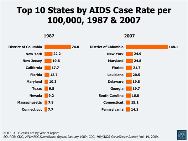
Top 10 States by HIV Rate 1987 and 2007 (CDC data)

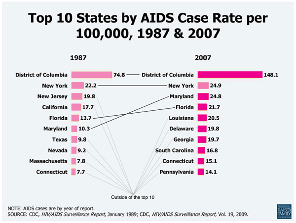
Top 10 States by HIV rate - modified

What Works

This data could easily have been thrown into a table – the bars make it a graphic. It is more visually interesting and instantly legible than a table, but are the bars enough?

What Needs Work

Most of the states on the top ten list in 1987 are not still on the list in 2007. That’s the most interesting part for me, and I would like the graphic to address that somehow — either by focusing on the four states that stayed on the list or by making sure it’s easy to see just how much movement there is on and off. What did the states at the top of the list in 1987 have in common? What about the states at the top in 2007? It appears that having a high percentage of the state living in urban areas makes some kind of difference but the graphic doesn’t give any clues at all about what is going on to get on or off the top ten list. Quite honestly, it doesn’t make sense to talk about the top ten states by HIV rate. It just doesn’t. That’s what the graph tells me.

I did try my hand at nudging the graphic in the right direction with the pink barred example. I don’t know if those converging lines pointing to somewhere outside the top ten help viewers to key into the large amount of movement on the list, but that is what I was thinking.

In the end, it would be better to go back to the data and come up with a more thoughtful analysis than to alter this graphic. The moral of the story is that the graphic can only be as helpful as the underlying data and the logic of the analysis.

Relevant Resources

CDC HIV Report – 2007

Centers for Disease Control. (2008) HIV/AIDS in the US – Factsheet

Kaiser Family Foundation. Topic: HIV/AIDS Fast Facts – Slides

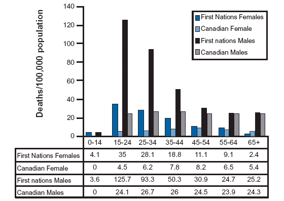
Crude Suicide Death Rate by Age Group - Canadian First Nations vs. All Canadians

What Works

I went looking for information about suicide and American Indian populations because I know that this is one indicator of the mental and physical health of a population. There is written work on American Indians out there, but this was the best information graphic on the subject and it happens to come from Canada where the population in question is referred to as First Nations. I like it because it respects that there has been (and continues to be) a difference in the rate of male and female suicide victims. Women tend to attempt suicide more often; men tend to be more successful in their attempts. I like it because it shows that the teen years are the most dangerous years for First Nations members by continuing the analysis across all age groups. They could have just truncated the graph at age 35 or so, since they are primarily concerned with the teen years, but instead they show the entire range of age cohorts. The viewer has to pick up on the fact that the difference between suicide rates of First Nations vs. all Canadian populations is most during the teen years and then falls off so dramatically that there is hardly any difference in old age. When viewers have to figure things out for themselves they are more likely to remember and trust those insights. I like that the tabular data is appended below the graph.

What Needs Work

Bar graphs are best when they are simple and this one is beginning to move away from simple. There are four bars for each cohort – it’s still legible, but it’s becoming hard to grasp the message at a glance with all those comparisons going on at once.

Relevant Resources

The North American Aboriginal Two Spirit Information Pages University of Calgary

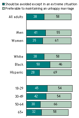
Pew Research Center  - Views on divorce
Pew Research Center - Views on divorce

Also in the original graphic: Notes: Whites include only non-Hispanic whites. Blacks include only non-Hispanic blacks. Hispanics are of any race. Don’t know responses are not shown.
Survey Date: February 16-March 14, 2007

What Works

This is one simple way to display data that is supposed to add up to 100%. It doesn’t work well when there are more than two categories, but I would rather see two categories like this than see two categories in pie charts. Two category pie charts often end up looking like pac man which could be particularly unfortunate when it is divorce data that is being displayed.

What Needs Work

I don’t understand why there are colors here. Shades of gray are just fine and would give the graphic a cleaner look overall. More importantly, I am unsure that it makes sense to portray age, race, and gender as the same kinds of data. From a strictly technical perspective, age is ordinal data here but race and gender are nominal data. More broadly, thinking that gender and race and age are having similar impacts on how people feel about divorce just doesn’t make sense.

Another thing that bothers me is the missing data. Sure, there’s a disclaimer than don’t know answers aren’t displayed, but I kept fixating on the fact that the numbers didn’t add up to 100 as they should. I would show those don’t know’s since not knowing how you feel about divorce seems like a piece of data to me, not just something someone forgot. I can forget a behavior (like whether or not I locked the door behind me this morning) but I can’t very easily forget an attitude. I have trouble, for example, forgetting how I feel about leaving an unhappy marriage. It’s also hard to use an “I forget” response when the question has been posed. If you’ve forgotten, now’s the time to remember! How about it, marriage forever or leaving if you’re pretty sure you’d be better off alone? The point is, saying “I don’t know” to this question is a key data point, not just a trivial lapse of memory about what a behavior.

Relevant Resources

Pew Research Center Social and Demographic Trends Views about Divorce by Age, Race and Gender

amazon.com, walmart.com, target.com, kmart.com
City Data
City Data

What Works

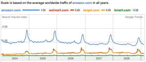
This is a graphic generated by one of google’s trend analysis tools. I simply typed in the web addresses I was curious about and google graphed their relative traffic patterns, using the first page I entered to set the scale. In their words, this is what the tool does: “Google Trends analyzes a portion of Google web searches to compute how many searches have been done for the terms you enter, relative to the total number of searches done on Google over time. “ If I were you, I would ignore the value of the scale and just keep in mind that it is relative. We’re measuring not total volume, but the volume of these four sites relative to one another.

Amazon clearly has far more traffic than the other three sites. Because walmart, target, and kmart rely on their physical stores, just looking at this web traffic does not tell you much about relative sales. I don’t who else is like me, but I often use amazon as a sort of loosely organized reference site, finding it faster to look their for publication dates of books than to go to my library’s site or fish the book off my shelf. I might be an outlier in this regard – most people don’t spend time every day wondering about publication dates – but there is probably a fair amount of traffic on amazon related to their product reviews that may not result in sales at amazon. All of this activity generates traffic, not sales. All three of the other retailers also feature customer reviews, by the way.

What works here is sort of unclear. On the one hand, just look at how similar walmart.com and target.com are. They track each other so closely they are visually difficult to distinguish. And just look at how important the holidays are to all these retailers.

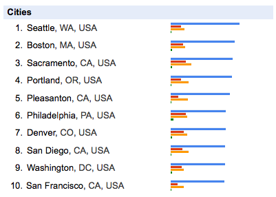
The city data relies heavily on which website is input into the search field first. Seattle might not have even been included if I had put walmart.com first, but many cities in the south would have been. Minneapolis would be up there if I had put target.com first. kmart.com first motivates Philly to the front of the pack.

What Needs Work

My biggest critique of this sort of thing is that it’s unclear what the heck to take from it. If you are just trying to beat some competitor, having google show you their relative traffic is immensely useful. But what else is this good for? Anyone?

Let me just point out that this only works for large sites. Google can’t tell us much about the vast sea of smaller sites.

Open Access – Transparency

In the end, though, the move towards making data publicly available is fabulous. I can’t see how this particular instance is broadly useful to me – it’s fascinating, sure, could be good for marketing departments internal to these companies, but then what? My confusion just means that I am a short-sighted fool. Google should be applauded for creating a non-prescriptive tool to explore the data they have that is so basic it can be used by anyone for who knows what.

Relevant Resources

Benkler, Y. (2006) The Wealth of Networks: How Social production Transforms Markets and Freedom. New Haven: Yale University Press.

Google Trends Information.

Google Trends the digital widget or digi-wigi.

Himanen, P. (2001) The Hacker Ethic. New York: Random House.

Raymond, E. (2001) The Cathedral & the Bazaar: Musings on Linux and Open Source by an Accidental Revolutionary. Sebastopol, CA: O’Reilly Media.

US Milk Production 1980 and 2003 by Region

What Works

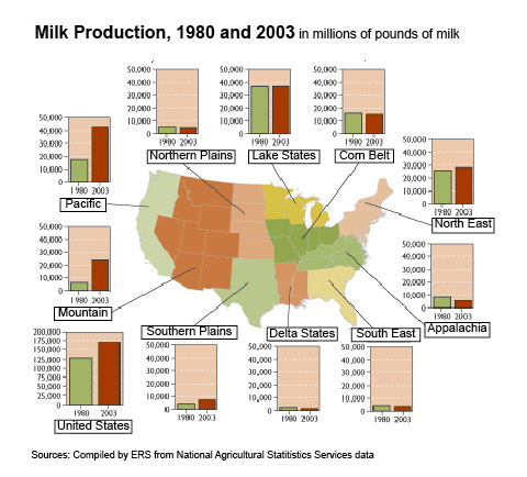
The first map was produced by the USDAs Economic Research Service in 2004 to show the change in milk production by US region from 1980 – 2003. The accompanying text is surprisingly brief, “Since 1980, milk production in the U.S. has increased almost 33 percent. Regional production growth has been most pronounced in the Pacific and Mountain regions, the result of development of low-cost systems of milk production in the Pacific region and some Mountain States. Growth has been much slower in the Northeast and Southern Plains, and the other six regions have seen essentially flat or declining production.”

The graphic is a fairly straightforward way to combine a map with a bar graph. I like it better than if it were just a bar graph with regional labels, but I would like it even more if it were better integrated so that the data from the graphs were embedded in the map, maybe by showing the change in production by color or by applying concavity/convexity to the map.

What Needs Work

There is a serious drawback to the map + graph combination. One of the problem with images is that they tend to appear as sealed, complete narratives that are telling the whole story. It’s hard to interrogate an image, harder than interrogating a text. We’re taught not to believe everything we read, but those strategies don’t translate directly into the world of images. The important missing information here is that the population in the US is shifting to the south and west out of the north east. The image doesn’t suggest causal links; but the text does. However, it leaves out the no-brainer that since milk is a localized commodity, population growth is generally going to result in increased milk production in that area.

US Population Change, 1970-2030

Bonus Image

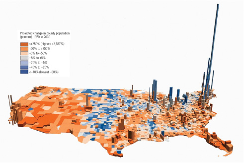
I found this image depicting population density and population change in the US. Cool colors indicate a loss of population; warm ones suggest growth. The z-axis represents human volume. A solid graphic. I have looked and looked and been unable to find the original source which just goes to show that once information hits the digital domain it really does have a life of its own. Hackers were right about that, information wants to be free.

Relevant Resources

Blayney, Donald. (2004) Milk production shifts West USDA Economic Research Center.

Dupuis, E. Melanie. (2002) Nature’s Perfect Food: How Milk Became America’s Drink. New York: NYU Press.

Mendelson, Anne. (2008) Milk: The Surprising Story of Milk Through the Ages. Knopf.

Figure 1 from "Diet, Energy, and Global Warming" by Eshel and Martin

US Greenhouse Gas Inventory Report - Executive Summary, Figure ES-11

Why This?

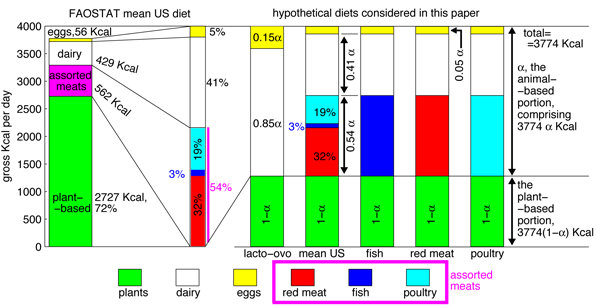
Continuing what I have decided will be an agriculture theme for the week, I went looking for data related to energy efficiency of diets. This concept first became news in the 1970’s during the energy crisis, championed in the book “Diet for a Small Planet” by Frances Moore Lappé which has recently been released as a 20th anniversary edition. I was interested in getting to the bottom of the planetary (rather than the personal) part of her argument which is that to produce unit weight of protein in the form of beef/veal, the animal is going to need an input equivalent to 21 units of protein and we’d be globally better off if we just ate the plant sources ourselves in terms of energy consumption and intelligent stewardship of the planet. I didn’t quite find what I was looking for to back up that data (yet) but I did find the contemporary twist on that argument which relates dietary choice to greenhouse gas emissions.

What Works

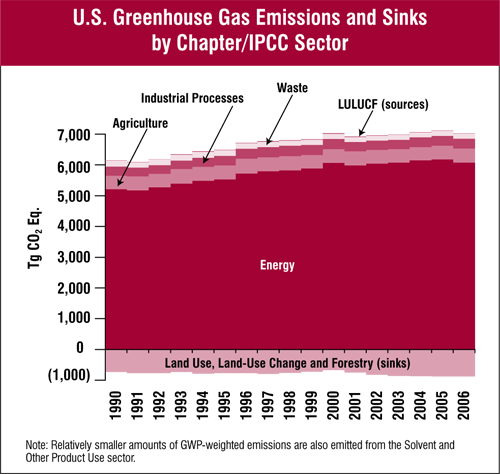
The first graphic doesn’t work all that well and probably makes no sense to you so we’ll come back to that. The second graphic, from the EPA, is not particularly pretty, but it has strength in simplicity and it makes intelligent use of the x-axis to represent greenhouse gas sinks. (Note: The visual representation does a great job of communicating that are emissions dwarf our sinks better than reading a number on a page would do.) Whereas the first graphic fails miserably to represent the difference in the energy efficiency of diets, the second graphic at least conveys the conclusion of the report that went along with the first graphic which is that the difference between eating the standard American diet and a vegan diet is, “far from trivial, …[it] amounts to over 6% of the total U.S. greenhouse gas emissions.”

The details of the report accompanying the first graphic are worth perusing and I only wish they would have spent more time trying to represent them graphically. The authors, Eshel and Martin, compute the comparative impacts of transit choice vs. dietary choice and find that, “while for personal transportation the average American uses 1.7 × 10⁷–6.8 × 10⁷ BTU yr−1, for food the average American uses roughly 4 × 10⁷ BTU yr−1.” That would make an excellent graphic in about ten different ways and catapult them past the problem that many readers are going to get tripped up looking at the orders of magnitude and units and miss the point.

What Needs Work

The first graphic is supposed to show the composition of the hypothetical diets considered. The mean American diet as reported by FAOSTAT has a little break-out component that provides more detail about the constituents of the animal products category but it took me a long hard look to figure that out. The break out part should have been constructed so it wasn’t exactly the same scale as the rest of the graphic (which it isn’t, by the way) otherwise it just reads like another column with viewers liable to assume that they can follow the scale on the y-axis. But the y-axis doesn’t relate to the break-out part at all – only the percentages listed alongside it are salient.

My bigger problem with the first graphic are the next five bars. Just to help you navigate α represents the proportion of the standard 3744 kcal diet that comes from animal sources. See α, think animal. A key would have been nice. Now that you know that, looking at the graph, it appears that each of the diets gets the same amount of kcals from plant sources because the green segments are all the same size. However, this is not actually what the authors are trying to convey. You have to read through the text quite carefully to pick out what proportion of each diet comes from animal sources overall. Once having done that, this graphic can help you further breakdown how those animal sources are apportioned. For example, the ovo-lacto group gets none of their animal protein from animal flesh – only from dairy (.85 of animal protein total) and eggs (.15 of animal protein total). But it took a good ten minutes of going between text and graphic to figure out what they have charted here. In all honesty, I’m still a little confused about whether the last three diets just switch out fish for meat for poultry and keep the same total number of kcalories in the animal flesh category relative to dairy+eggs. And I certainly can’t tell if any of those hypothetical diets have a greater or lesser proportion of kcals coming from plants by looking at this graphic.

In summary, the two graphics here were not trying to make the same point. The first one was trying to explain how the authors modeled their hypothetical diets in order to convince you that, in the end, and in conjunction with some other writing and graphic representation, if Americans moved to vegan diets the national greenhouse gas emission rate would drop by 6%, on par with what would happen if everyone started driving a Prius. The second graphic does this much better using aggregate data (and thus a totally different approach than Eshel and Martin).

Relevant Resources

Eshel, Gidon and Martin, Pamela. (May 2005) Diet, Energy and Global Warming. Submitted to Earth Interactions.

United States Environmental Protection Agency. (April 2008) Inventory of U.S. Greenhouse Gas Emissions and Sinks: 1990-2006

Moore Lappé, Frances. (1971, 1991) Diet for a Small Planet Ballantine Books.